References (utilities and misc)

General tools

misc utilities

download(url, output)

Download a file from a given URL using asynchronous HTTP requests.

Parameters:

• url (str) -- The URL from which to download the file.

• output (str) -- The path and filename where the downloaded file will be saved.

Raises a KeyboardInterrupt or asyncio.TimeoutError if the download is interrupted or takes too long. In such cases, it logs a message, removes partially downloaded files, and logs a critical message.

findpos(seq, chr)

Find position(s) of a substring into a longer string.

Note that this function is a generator:

>>> list(findpos("AACCGGAAGGTT", "GG"))
[4,8]

multiple_downloads(files_to_download, timeout=3600)

normpdf(x, mu, sigma)

Return the normal pdf evaluated at x; args provides mu, sigma"

Note

same as scipy.stats.norm but implemented to avoid scipy dependency

textwrap(text, width=80, indent=0)

Wrap a string with 80 characters

Parameters:

• text -- input text

• width -- (defaults to 80 characters)

• indent -- possible indentation (0 by default)

wget(link, output)

Retrieve a file from internet.

Parameters:

• link (str) -- a valid URL

• output (str) -- the output filename

Warning

no sanity check of any kind for now

General tools

class GZLineCounter(filename)

Fast GZipped line counter

Uses zcat if possible, otherwise gzip library (twice as slow).

>>> from sequana import sequana_data
>>> from sequana.tools import GZLineCounter
>>> gz = GZLineCounter(sequana_data("test.fastq.gz"))
>>> len(gz)
1000

class StatsBAM2Mapped(bamfile=None, wkdir=None, verbose=True)

to_html()

to_json(filename)

bam_to_mapped_unmapped_fastq(filename, output_directory=None, progress=True)

Create mapped and unmapped fastq files from a BAM file

Context:

given a reference, one or two FastQ files are mapped onto the reference to generate a BAM file. This BAM file is a compressed version of a SAM file, which interpretation should be eased within this function.

Parameters:

• filename -- input BAM file

• output_directory -- where to save the mapped and unmapped files

Returns:

dictionary with number of reads for each file (mapped/unmapped for R1/R2) as well as the mode (paired or not), the number of unpaired reads, and the number of duplicated reads. The unpaired reads should be zero (sanity check)

Given a BAM file, create FASTQ with R1/R2 reads mapped and unmapped. In the paired-end case, 4 files are created.

Note that this function is efficient in that it does not create intermediate files limiting IO in the process. As compared to standard tools such as bedtools bamtofastq, it is 1.5 to 2X slower but it does create the mapped AND unmapped reads.

Details:

Secondary alignment (flag 256) are dropped so as to remove any ambiguous alignments. The output dictionary stores "secondary" key to keep track of the total number of secondary reads that are dropped. If the flag is 256 and the read is unpaired, the key unpaired is also incremented.

If the flag is not equal to 256, we first reverse complement reads that are tagged as reverse in the BAM file. Then, reads that are not paired or not "proper pair" (neither flag 4 nor flag 8) are ignored.

If R1 is mapped or R2 is mapped then the reads are considered mapped. If both R1 and R2 are unmapped, then reads are unmapped.

Note

about chimeric alignment: one is the representative and the other is the supplementary. This flag is not used in this function. Note also that chimeric alignment have same QNAME and flag 4 and 8

Note

the contamination reported is based on R1 only.

Todo

comments are missing since there are not stored in the BAM file.

Note

the mapped reads may not be synchronized because we include also the chimeric alignment (cf samtools documentation). However, total reads = unmappeds reads + R1 mapped + R2 mapped - supplementary reads (those with flag 2048).

compute_bendability(seq, scale, window=3)

DNA bendability measures the local flexibility of a DNA sequence—its ability to bend or deform. This is a crucial feature in:

Brukner et al. (1995)

compute_helix_twist(seq, scale)

Helix twist refers to the rotational angle between adjacent base pairs in the DNA double helix, typically measured in degrees. It reflects how tightly the DNA is twisted and is important for:

• DNA supercoiling

• Protein-DNA interactions

• Nucleosome positioning

• Local helical structure variations (e.g., bends, kinks)

Typical Values: Canonical B-DNA: ~36° per base pair step Varies with sequence: ~32°–40° depending on dinucleotide

lempel_ziv_complexity(seq)

Lempel-Ziv complexity is a measure of sequence compressibility—how "random" or "repetitive" a sequence is. In the context of DNA, it captures how diverse the patterns are. A low LZ complexity suggests repeats or low complexity regions, while a high LZ complexity suggests a more random or information-rich sequence.

Manipulate phred quality of reads

FastQ quality are stored as characters. The phred scales indicates the range of characters.

In general, characters goes from ! to ~ that is from 33 to 126 in an ascii table. This convention starts at 33 because characters before ! may cause trouble (e.g. white spaces). This scale is the Sanger scale. There are 2 other scales that could be used ranging from 59 to 126 (illumina 1) and from 64 to 126 (illumina 1.3+).

So, here are the offset to use:

Name	offset	Numeric range
Sanger	33	0 to 93
Solexa	64	-5 to 62
illumina1.3+	64	0 to 62

reference:

http://www.ncbi.nlm.nih.gov/pmc/articles/PMC2847217/

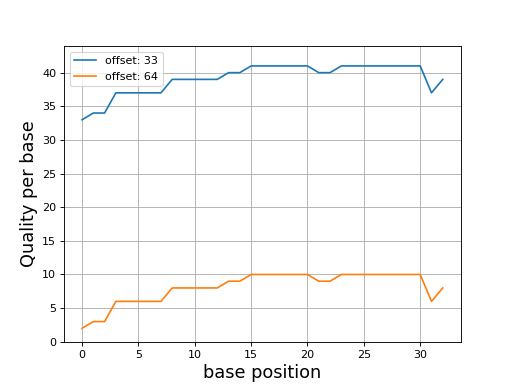
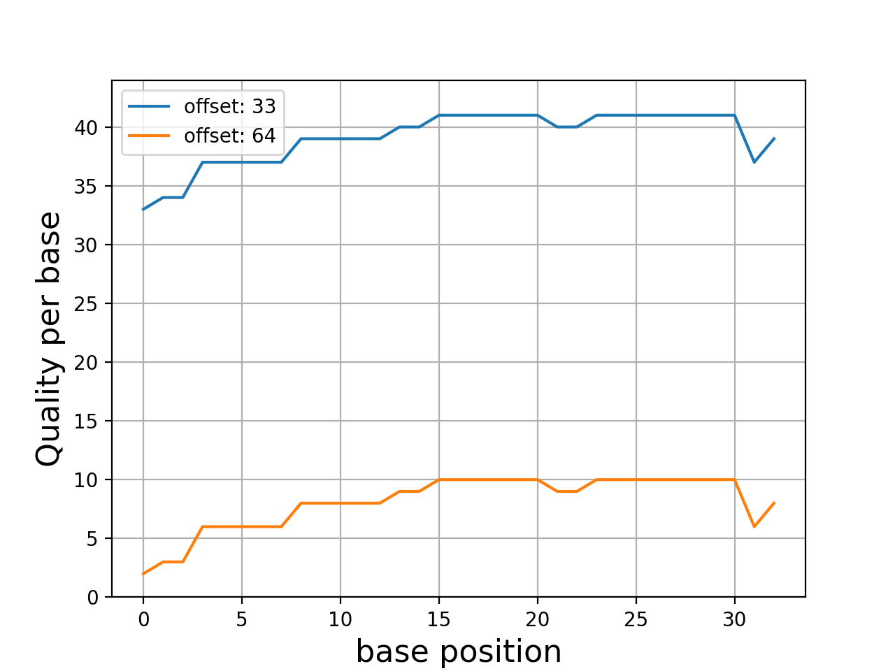
Even though dedicated tools would have better performances, we provide a set of convenient functions. An example is provided here below to plot the quality corresponding to a character string extracted from a FastQ read.

In this example, we use Quality class where the default offset is 33 (Sanger). We compare the quality for another offset

from sequana import phred

from sequana.phred import Quality
q = Quality('BCCFFFFFHHHHHIIJJJJJJIIJJJJJJJJFH')
q.plot()
q.offset = 64
q.plot()
from pylab import legend
legend(loc="best")

(Source code, png, hires.png, pdf)

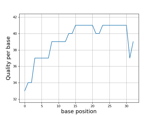
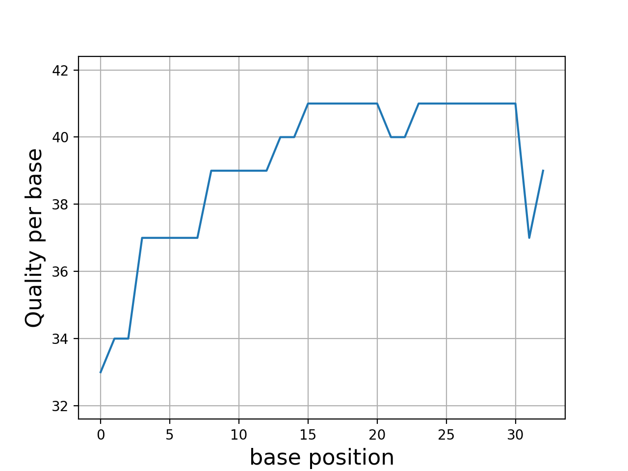
class Quality(seq, offset=33)

Phred quality

>>> from sequana.phred import Quality
>>> q = Quality('BCCFFFFFHHHHHIIJJJJJJIIJJJJJJJJFH')
>>> q.plot()

(Source code, png, hires.png, pdf)

You can access to the quality as a list using the quality attribute and the mean quality from the mean_quality attribute.

property mean_quality

return mean quality

plot(fontsize=16)

plot quality versus base position

property quality

phred string into quality list

proba_to_quality_sanger(pe)

A value between 0 and 93

Parameters:

pe -- the probability of error.

Returns:

Q is the quality score.

• a high probability of error (0.99) gives Q=0

• q low proba of errors (0.05) gives Q = 13

• q low proba of errors (0.01) gives Q = 20

quality_to_proba_sanger(quality)

Quality to probability (Sanger)

simple summary class to handle summary data with metadata

class Summary(name, sample_name='undefined', data={}, caller=None, pipeline_version=None)

>>> s = Summary("test", "chr1", data={"mean": 1})
>>> s.name
sequana_summary_test
>>> s.sample_name
chr1

Here, we prefix the name with the "sequana_summary" tag. Then, we populate the sequana version and date automatically. The final summary content is then accessible as a dictionary:

>>> s.as_dict()
{'data': {'mean': 1},
 'date': 'Thu Jan 18 22:09:13 2018',
 'name': 'sequana_summary_test',
 'sample_name': 'chr1',
 'version': '0.6.3.post1'}

You can also populate a description dictionary that will provide a description for the keys contained in the data field. For instance, here, the data dictionary contains only one obvious field (mean), we could provide a description:

s.data_description = {"mean": "a dedicated description for the mean"}

A more general description can also be provided:

s.description = "bla bla bla"

add_params(params)

as_dict()

property data_description

property date

property name

to_json(filename)

property version

Test data and discovery

Retrieve data from sequana library

sequana_data(filename=None, where=None)

Return full path of a sequana resource data file.

Parameters:

• filename (str) -- a valid filename to be found

• where (str) -- one of the registered data directory (see below)

Returns:

the path of file. See also here below in the case where filename is set to "*".

from sequana import sequana_data
filename = sequana_data("test.fastq")

Type the function name with "*" parameter to get a list of available files. Withe where argument set, the function returns a list of files. Without the where argument, a dictionary is returned where keys correspond to the registered directories:

filenames = sequana_data("*", where="images")

Registered directories are:

• data

• testing

• images

Note

this does not handle wildcards. The * means retrieve all files.

Some useful data sets to be used in the analysis

The command sequana.sequana_data() may be used to retrieved data from this package. For example, a small but standard reference (phix) is used in some NGS experiments. The file is small enough that it is provided within sequana and its filename (full path) can be retrieved as follows:

from sequana import sequana_data
fullpath = sequana_data("phiX174.fa", "data")

Other files stored in this directory will be documented here.

adapters = {'adapters_netflex_pcr_free_1_fwd': 'adapters_netflex_pcr_free_1_fwd.fa', 'adapters_netflex_pcr_free_1_rev': 'adapters_netflex_pcr_free_1_rev.fa'}

List of adapters used in various sequencing platforms

sequana.utils

Utilities to create a Jquery DataTable for your HTML file.

DataTableFunction(df, html_id[, index])	Class that contains Jquery DataTables function and options.
DataTable(df, html_id[, datatable, index])	Class that contains html table which used a javascript function.

class DataTable(df, html_id, datatable=None, index=False)

Class that contains html table which used a javascript function.

You must add in your HTML file the JS function (DataTable.create_javascript_function()) and the HTML code (DataTable.create_datatable()).

Example:

df = pandas.read_csv('data.csv')
datatable = DataTable(df, 'data')
datatable.datatable.datatable_options = {'pageLength': 15,
                                         'dom': 'Bfrtip',
                                         'buttons': ['copy', 'csv']}
js = datatable.create_javascript_function()
html = datatable.create_datatable()

# Second CSV file with same format
df2 = pandas.read_csv('data2.csv')
datatable2 = DataTable(df2, 'data2', datatable.datatable)
html2 = datatable.create_datatable()

The reason to include the JS manually is that you may include many HTML table but need to include the JS only once.

contructor

Parameters:

• df -- data frame.

• html_id (str) -- the unique ID used in the HTML file.

• datatable (DataTableFunction) -- javascript function to create the Jquery Datatables. If None, a DataTableFunction is generated from the df.

• index (bool) -- indicates whether the index dataframe should be shown

create_datatable(style='width:100%', **kwargs)

Return string well formated to include in a HTML page.

Parameters:

• style (str) -- CSS option of your table.

• kwargs (dict) -- parameters of pandas.DataFrame.to_csv().

create_javascript_function()

Generate the javascript function to create the DataTable in a HTML page.

property df

property html_id

class DataTableFunction(df, html_id, index=False)

Class that contains Jquery DataTables function and options.

Example:

import pandas as pd
from sequana.utils.datatables_js import DataTableFunction

df = pandas.read_csv('data.csv')
datatable_js = DataTableFunction(df, 'data')
datatable_js.datatable_options = {'pageLength': 15,
                                  'dom': 'Bfrtip',
                                  'buttons': ['copy', 'csv']}
js = datatable_js.create_javascript_function()
html_datatables = [DataTable(df, "data_{0}".format(i), datatable_js)
                   for i, df in enumerate(df_list)]

Here, the datatable_options dictionary is used to fine tune the appearance of the table.

Note

DataTables add a number of elements around the table to control the table or show additional information about it. There are controlled by the order in the document (DOM) defined as a string made of letters, each of them having a precise meaning. The order of the letter is important. For instance if B is first, the buttons are put before the table. If B is at the end, it is shown below the table. Here are some of the valid letters and their meaning:

• B: add the Buttons (copy/csv)

• i: add showing 1 to N of M entries

• f: add a search bar (f filtering)

• r: processing display element

• t: the table itself

• p: pagination control

Each option can be specified multiple times (with the exception of the table itself).

Note

other useful options are:

• pageLength: 15

• scrollX: "true"

• paging: 15

• buttons: ['copy', 'csv']

Note that buttons can also be excel, pdf, print, ...

All options of datatable:

https://datatables.net/reference/option/

contructor

Parameters:

• df -- data frame.

• html_id (str) -- the ID used in the HTML file.

create_javascript_function()

Return javascript to create the DataTable.

property datatable_columns

Get datatable_columns dictionary. It is automatically set from the dataframe you want to plot.

property datatable_options

Get, set or delete the DataTable options. Setter takes a dict as parameter with the desired options and updates the current dictionary.

Example:

datatable = DataTableFunction("tab")
datatable.datatable_options = {'dom': 'Bfrtip',
                               'buttons': ['copy', 'csv']}

source: https://datatables.net/reference/option/

property html_id

Get the html_id, which cannot be set by the user after the instanciation of the class.

set_links_to_column(link_col, target_col, new_page=True)

Hide a column with urls and connect it with a column.

Parameters:

• link_col (str) -- column with your URLs.

• target_col (str) -- column to connect.

set_tooltips_to_column(tooltips_col, target_col)

Hide a column with tooltips and connect it with a column.

Parameters:

• tooltips_col (str) -- column with your tooltips.

• target_col (str) -- column to connect.

class Checker

Utility to hold checks

The method /tryme() calls the method or function provided. This method is expected to return a dictionary with 2 keys called status and msg. Status should be in 'Error', 'Warning', 'Success'.

The attributes hold all calls to tryme()

Given that func returns a dictionary as explained here above, you can run this code

checks = Checker()
checks.tryme(func)

checks contains the status and mesg of each function called by checks.tryme.

tryme(meth)

Sequana report config contains configuration informations to create HTML report with Jinja2.

df2html(df, name=None, dom='Brt', show_index=False, pageLength=15)

Simple wrapper to create HTML from dataframe

If a columns ends in _links and a name_links exists, then the columns name will be shown with the clickable name_links.

fisher_exact(array_2by2, alternative)

Fast Fisher test alternative to scipy

lgamma(z)

mlnTest2l(a, ab, ac, abcd)

mlnTest2r(a, ab, ac, abcd)

mlnTest2t(a, ab, ac, abcd)

test_both(a, b, c, d)

test_left(a, b, c, d)

test_right(a, b, c, d)

Simple utilities for pandas

class PandasReader(filename, sep='\t', columns=None, **kwargs)

class Singleton

class DisplayablePath(path, parent_path, is_last)

paths = DisplayablePath.make_tree(Path('doc'))
for path in paths:
    print(path.displayable())

Inspired from https://stackoverflow.com/questions/9727673/list-directory-tree-structure-in-python

display_filename_prefix_last = '└──'

display_filename_prefix_middle = '├─'

display_parent_prefix_last = '│   '

display_parent_prefix_middle = '    '

displayable()

property displayname

classmethod make_tree(root, parent=None, is_last=False, criteria=None)

class HTMLDirectory(path='.', skip_pattern=[], pattern=None)

get_html()

sequana.plots

Base class for CanvasJS plot to set legend, title, axis and commun things.

class CanvasJS(html_id)

Base class to create any type of graph with CanvasJS.

constructor

Parameters:

html_id (str) -- the ID used in your html. All function will have this tag.

create_canvas_js_object()

Method to convert all section as javascript function. Return string.

create_div_chart_container(style_option='')

HTML div that contains CanvasJS chart.

Parameters:

style_option (str) -- css option for your chart.

return a string.

set_data(data_dict, index=None)

Method to convert dictionnarie as data field for CanvasJS.

Parameters:

• data_attr (dict) -- dictionary with CanvasJS data attributes.

• index (int) -- which data you want to update.

data: http://canvasjs.com/docs/charts/chart-options/data/

Populate CanvasJS.data_section.

set_legend(legend_attr={}, hide_on_click=True)

Method to configure legend of the CanvasJS chart.

Parameters:

legend_attr (dict) -- dictionary with CanvasJS legend attributes.

legend: http://canvasjs.com/docs/charts/chart-options/legend/

Example:

canvasjs = CanvasJS()
canvasjs.set_legend({'fontFamily': 'verdana',
                     'fontSize': 12,
                     'verticalAlign': 'bottom'}

Populate the dictionary legend_section.CanvasJS.

set_options(options={})

Method to add options for the CanvasJS chart.

Parameters:

options (dict) -- dictionary with desired options for CanvasJS.

options: http://canvasjs.com/docs/charts/chart-options/

Populate the dictionary CanvasJS.options.

set_title(title, title_attr={})

Method to configure title of the CanvasJS chart.

Parameters:

• title (str) -- title of the chart.

• title_attr (dict) -- canvasjs title attributes

title: http://canvasjs.com/docs/charts/chart-options/title

Example:

canvasjs = CanvasJS()
canvasjs.set_title("Title of the plot", {'fontFamily': 'verdana',
                                         'fontSize': 16,
                                         'verticalAlign': 'top'})

Populate CanvasJS.title_section

Sequana class to plot a CanvasJS linegraph from an embedded csv file.

class CanvasJSLineGraph(csv, html_id, x_column, y_columns)

Class to create a CanvasJS linegraphe for an HTML page. It creates a hidden pre section with your CSV. It is necessary embedded because browsers forbid the reading of data stored locally. Your html page need CanvasJS and PapaParse.

constructor

Parameters:

• csv (str) -- data as CSV format.

• html_id (str) -- the ID used in your html. All function will have this tag.

• x_column (str) -- column used as axis X for plot.

• y_columns (list) -- colums used as axis Y for plot.

create_canvasjs()

Method to convert all section as javascript function.

Return a string which contains command line to launch generation of plot, js function to create CanvasJS object and the html div that contains CanvasJS plot.

set_axis_x(axis_attr={})

Method to configure X axis of the line graph.

Parameters:

axis_attr (dict) -- dictionary with canvasjs axisX Attributes.

axisX: http://canvasjs.com/docs/charts/chart-options/axisx/

Example:

line_graph = CanvaJSLineGraph(csv, csvdata)
axisX_section = line_graph.set_x_axis({
    'title': 'Title of X data',
    'titleFontSize': 16,
    'labelFontSize': 12,
    'lineColor': '#5BC0DE',
    'titleFontColor': '#5BC0DE',
    'labelFontColor': '#5BC0DE'})

set_axis_y(axis_attr={})

Method to configure first axis Y of the line graph.

Parameters:

axis_attr (dict) -- dictionary with canvasjs axisY Attributes.

axisY: http://canvasjs.com/docs/charts/chart-options/axisy/

Example:

line_graph = CanvaJSLineGraph(csv, csvdata)
line_graph.set_y_axis({'title': 'Title of Y data',
                       'titleFontSize': 16,
                       'labelFontSize': 12,
                       'lineColor': '#5BC0DE',
                       'titleFontColor': '#5BC0DE',
                       'labelFontColor': '#5BC0DE'})

set_axis_y2(axis_attr={})

Method to configure second axis Y of the line graph.

Parameters:

axis_attr (dict) -- dictionary with canvasjs axisY Attributes.

axisY: http://canvasjs.com/docs/charts/chart-options/axisy/

Example:

line_graph = CanvaJSLineGraph(csv, csvdata)
axisX_section = line_graph.set_x_axis({
    'title': 'Title of Y data',
    'titleFontSize': 16,
    'labelFontSize': 12,
    'lineColor': '#5BC0DE',
    'titleFontColor': '#5BC0DE',
    'labelFontColor': '#5BC0DE'})