References (pipeline back-ends)#

BAM / alignment #

Tools to manipulate BAM/SAM files

`Alignment`(alignment)	Helper class to retrieve info about Alignment
`BAM`(filename, *args)	BAM reader.
`CRAM`(filename, *args[, reference_filename])	CRAM Reader.
`MultiBAM`()	Convenient structure to store several BAM files
`SAM`(filename, *args)	SAM Reader.
`SAMFlags`([value])	Utility to extract bits from a SAM flag
`SAMBAMbase`(filename[, mode])	Base class for SAM/BAM/CRAM data sets

Note

BAM being the compressed version of SAM files, we do not implement any functionalities related to SAM files. We strongly encourage developers to convert their SAM to BAM.

class Alignment(alignment)[source]#

Helper class to retrieve info about Alignment

Takes an alignment as read by BAM and provides a simplified version of pysam.Alignment class.

>>> from sequana.bamtools import Alignment
>>> from sequana import BAM, sequana_data
>>> b = BAM(sequana_data("test.bam"))
>>> segment = next(b)
>>> align = Alignment(segment)
>>> align.as_dict()
>>> align.FLAG
353

The original data is stored in hidden attribute _data and the following values are available as attributes or dictionary:

QNAME: a query template name. Reads/segment having same QNAME come from the same template. A QNAME set to * indicates the information is unavailable. In a sam file, a read may occupy multiple alignment
FLAG: combination of bitwise flags. See SAMFlags
RNAME: reference sequence
POS
MAPQ: mapping quality if segment is mapped. equals -10 log10 Pr
CIGAR: See sequana.cigar.Cigar
RNEXT: reference sequence name of the primary alignment of the NEXT read in the template
PNEXT: position of primary alignment
TLEN: signed observed template length
SEQ: segment sequence
QUAL: ascii of base quality

constructor

Parameters:: alignment -- alignment instance from BAM

as_dict()[source]#

Return alignment fields as an ordered dictionary.

Returns:: dict with keys QNAME, FLAG, RNAME, POS, MAPQ, CIGAR, PNEXT, RNEXT, TLEN, SEQ, and QUAL.
Return type:: dict

class BAM(filename, *args)[source]#

BAM reader. See SAMBAMbase for details

Initialise a BAM reader.

Parameters:

filename (str) -- path to the BAM file.
args -- additional arguments forwarded to SAMBAMbase.

class CRAM(filename, *args, reference_filename=None)[source]#

CRAM Reader. See SAMBAMbase for details

Initialise a CRAM reader.

Parameters:

filename (str) -- path to the CRAM file.
reference_filename (str) -- optional path to the reference FASTA file. Required when the path stored inside the CRAM header is not accessible (e.g. when running on a different machine than the one that created the file).
args -- additional arguments forwarded to SAMBAMbase.

class CS(tag)[source]#

Interpret CS tag from SAM/BAM file tag

>>> from sequana import CS
>>> CS('-a:6-g:14+g:2+c:9*ac:10-a:13-a')
{'D': 3, 'I': 2, 'M': 54, 'S': 1}

When using some mapper, CIGAR are stored in another format called CS, which also includes the substitutions. See minimap2 documentation for details.

Parse a CS tag string and store CIGAR-like counts.

Parameters:: tag (str) -- CS tag string as produced by minimap2 (e.g. "-a:6-g:14+g:2+c:9*ac:10").

class SAM(filename, *args)[source]#

SAM Reader. See SAMBAMbase for details

Initialise a SAM reader.

Parameters:

filename (str) -- path to the SAM file.
args -- additional arguments forwarded to SAMBAMbase.

class SAMBAMbase(filename, mode='r', *args, **kwargs)[source]#

Base class for SAM/BAM/CRAM data sets

We provide a few test files in Sequana, which can be retrieved with sequana_data:

>>> from sequana import BAM, sequana_data
>>> b = BAM(sequana_data("test.bam"))
>>> len(b)
1000
>>> from sequana import CRAM
>>> b = CRAM(sequana_data("test_measles.cram"))
>>> len(b)
60

Initialise a SAM/BAM/CRAM reader.

Parameters:

filename (str) -- path to the SAM, BAM, or CRAM file.
mode (str) -- pysam open mode. Use "r" for SAM/CRAM and "rb" for BAM (the default for BAM).
args -- additional positional arguments forwarded to pysam.AlignmentFile.
kwargs -- additional keyword arguments forwarded to pysam.AlignmentFile (e.g. reference_filename for CRAM files).

bam_analysis_to_json(filename)[source]#

Create a json file with information related to the bam file.

This includes some metrics (see get_stats(); eg MAPQ), combination of flags, SAM flags, counters about the read length.

boxplot_qualities(max_sample=500000)[source]#: Same as in sequana.fastq.FastQC

get_df(max_align=-1, progress=True, include_cigar=False)[source]#

Build a pandas.DataFrame with one row per alignment.

Columns include flags, mapq, start, end, rname (reference name), qname (query/read name), query_length, query_aln_length, and CIGAR-derived counts I (insertions), D (deletions), and M (matches), plus the number of mismatches (NM tag) and mismatch (NM normalised by alignment length).

Parameters:

max_align (int) -- maximum number of alignments to include. -1 means no limit.
progress (bool) -- show a tqdm progress bar. Defaults to True.
include_cigar (bool) -- include the raw CIGAR string in the returned dataframe. Defaults to False.

Returns:

DataFrame with one row per alignment.

Return type:

pandas.DataFrame

get_df_concordance(max_align=-1, progress=True)[source]#

This methods returns a dataframe with Insert, Deletion, Match, Substitution, read length, concordance (see below for a definition)

Be aware that the SAM or BAM file must be created using minimap2 and the --cs option to store the CIGAR in a new CS format, which also contains the information about substitution. Other mapper are also handled (e.g. bwa) but the substitution are solely based on the NM tag if it exists.

alignment that have no CS tag or CIGAR are ignored.

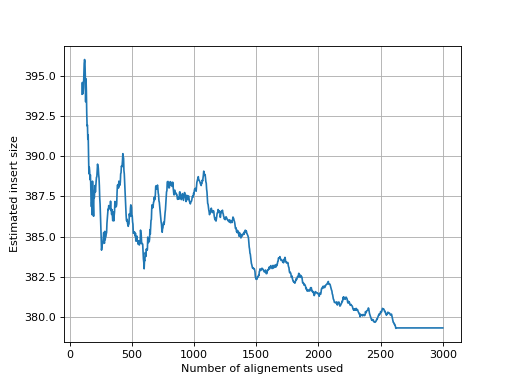
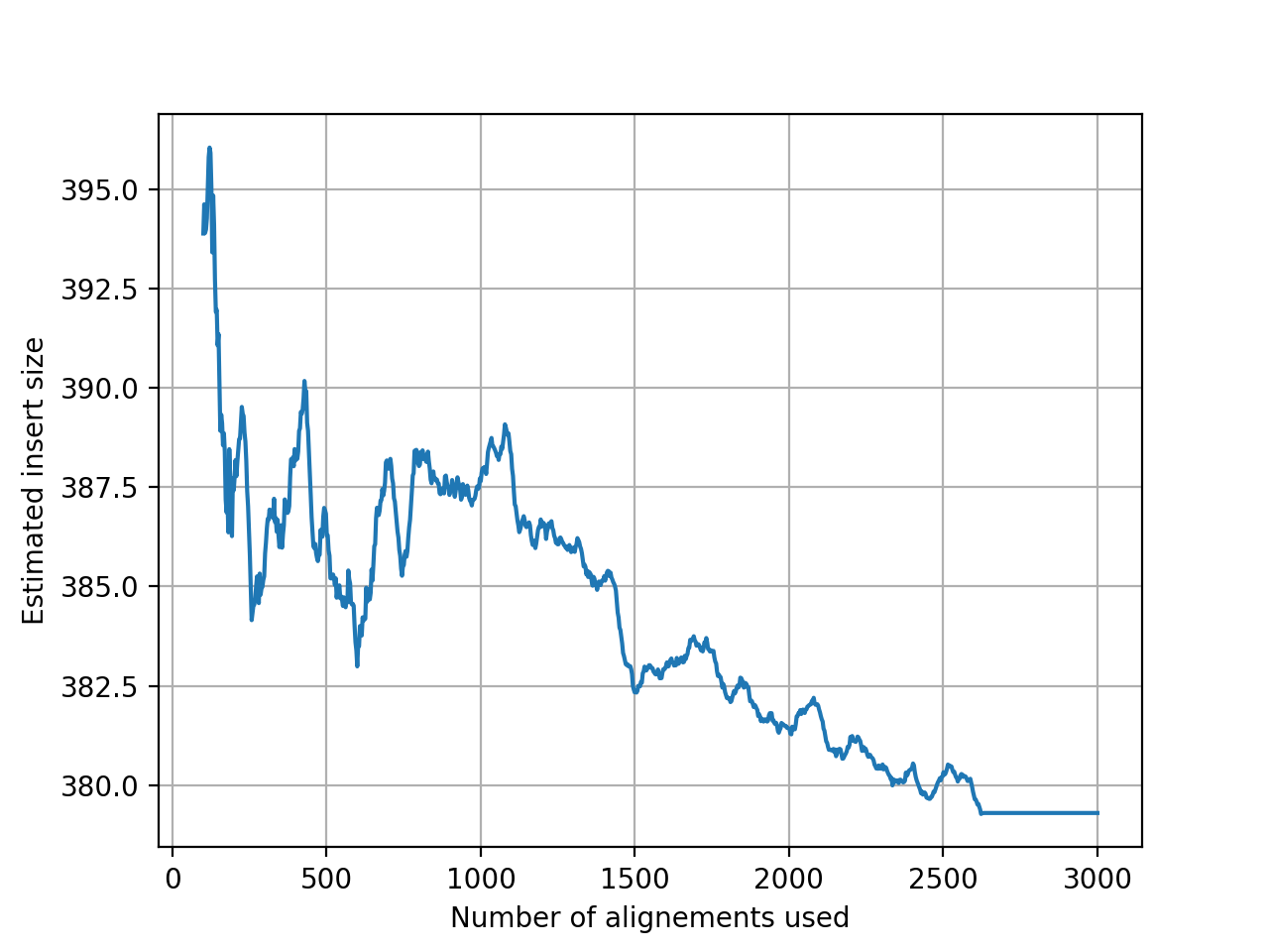
get_estimate_insert_size(max_entries=100000, upper_bound=1000, lower_bound=-1000)[source]#

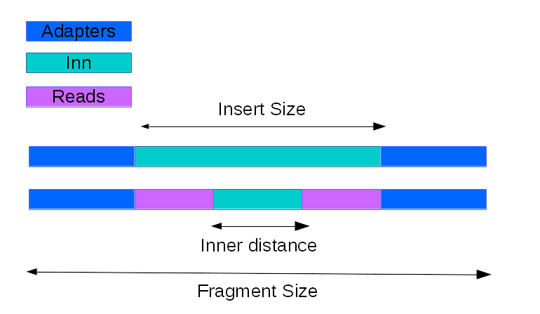
Here we show that about 3000 alignments are enough to get a good estimate of the insert size.

(Source code, png, hires.png, pdf)

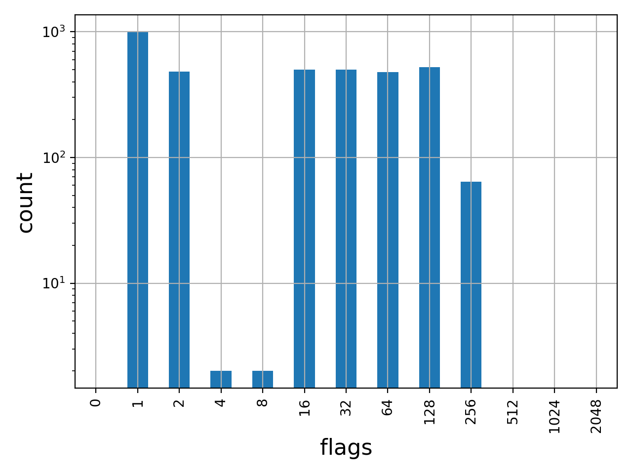
get_flags_as_df()[source]#

Returns decomposed flags as a dataframe

>>> from sequana import BAM, sequana_data
>>> b = BAM(sequana_data('test.bam'))
>>> df = b.get_flags_as_df()
>>> df.sum()
        0
     1000
      484
        2
        2
     499
     500
     477
    523
     64
      0
     0
     0
dtype: int64

See also

SAMFlags for meaning of each flag

get_gc_content()[source]#: Return GC content for all reads (mapped or not)

See also

plot_gc_content()

get_length_count()[source]#: Return counter of all fragment lengths

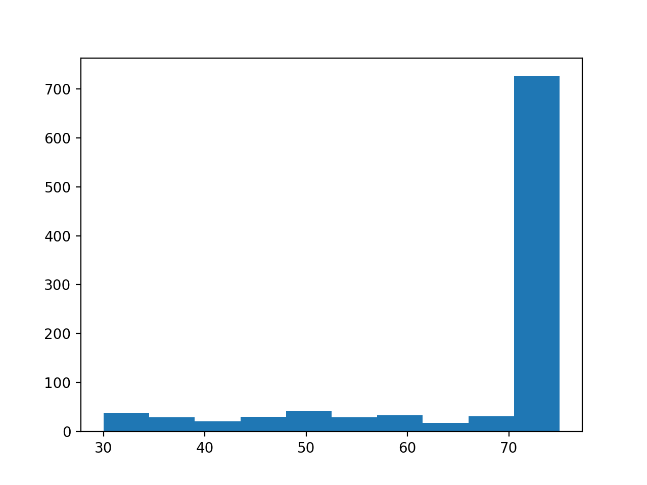
get_mapped_read_length()[source]#

Return dataframe with read length for each read

(Source code, png, hires.png, pdf)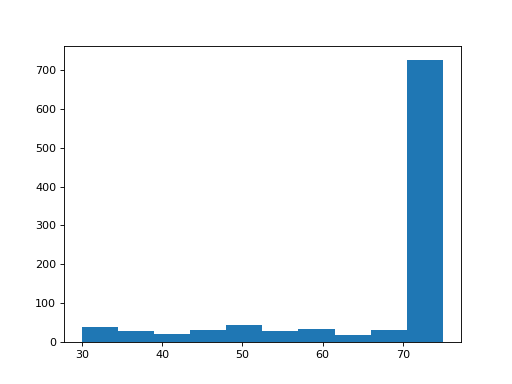

get_mapq_as_df(max_entries=-1)[source]#: Return dataframe with mapq for each read

get_query_end(read)[source]#: Get end of the query read.

get_query_start(read)[source]#: Get start of the query read.

get_read_names()[source]#: Return the reads' names

get_samflags_count()[source]#

Count how many reads have each flag of SAM format.

Returns:: dictionary with keys as SAM flags

get_samtools_stats_as_df()[source]#

Return a dictionary with full stats about the BAM/SAM file

The index of the dataframe contains the flags. The column contains the counts.

>>> from sequana import BAM, sequana_data
>>> b = BAM(sequana_data("test.bam"))
>>> df = b.get_samtools_stats_as_df()
>>> df.query("description=='average quality'")
36.9

Note

uses samtools behind the scene

get_stats()[source]#

Return basic stats about the reads

Returns:

dictionary with basic stats:

total_reads : number reads ignoring supplementaty and secondary reads
mapped_reads : number of mapped reads
unmapped_reads : number of unmapped
mapped_proper_pair : R1 and R2 mapped face to face
reads_duplicated: number of reads duplicated

Warning

works only for BAM files. Use get_samtools_stats_as_df() for SAM files.

get_stats_full(mapq=30, max_entries=-1)[source]#

Compute detailed alignment statistics in a single pass over the BAM file.

This is a pure-Python implementation that does not rely on samtools directly, although it uses pysam for reading the file. It is slower than samtools flagstat but produces a richer set of metrics.

Parameters:

mapq (int) -- minimum mapping quality to consider a read as uniquely mapped. Defaults to 30.
max_entries (int) -- stop after this many alignments. -1 means process the entire file. Defaults to -1.

Returns:

dict with keys such as average_quality, average_length, forward, reverse, unmapped, reads_paired, mismatches, splice, non_splice, proper_pair, secondary, reads_duplicated, etc.

Return type:

dict

Note

On a typical BAM file this takes around 7 minutes. For a faster (but less detailed) summary use get_stats().

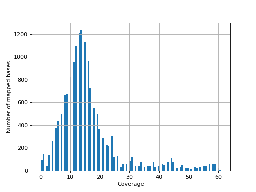
hist_coverage(chrom=None, bins=100)[source]#

from sequana import sequana_data, BAM
b = BAM(sequana_data("measles.fa.sorted.bam"))
b.hist_coverage()

(Source code, png, hires.png, pdf)

hist_soft_clipping()[source]#: histogram of soft clipping length ignoring supplementary and secondary reads

infer_strandness(reference_bed, max_entries, mapq=30)[source]#

Parameters:

reference_bed -- a BED file (12-columns with columns 1,2,3,6 used) or GFF file (column 1, 3, 4, 5, 6 are used
mapq -- ignore alignment with mapq below 30.
max_entries -- can be long. max_entries restrict the estimate

Strandness of transcript is determined from annotation while strandness of reads is determined from alignments.

For non strand-specific RNA-seq data, strandness of reads and strandness of transcript are independent.

For strand-specific RNA-seq data, strandness of reads is determined by strandness of transcripts.

This functions returns a list of 4 values. First one indicates whether data is paired or not. Second and third one are ratio of reads explained by two types of strandness of reads vs transcripts. Last values are fractions of reads that could not be explained. The values 2 and 3 tell you whether this is a strand-specificit dataset.

If similar, it is no strand-specific. If the first value is close to 1 while the other is close to 0, this is a strand-specific dataset

property is_paired#: Return True if the first read in the file is paired-end.

property is_sorted#: return True if the BAM is sorted

mRNA_inner_distance(refbed, low_bound=-250, up_bound=250, step=5, sample_size=1000000, q_cut=30)[source]#

Estimate the inner distance of mRNA pair end fragment.

from sequana import BAM, sequana_data
b = BAM(sequana_data("test_hg38_chr18.bam"))
df = b.mRNA_inner_distance(sequana_data("hg38_chr18.bed"))

plot_bar_flags(logy=True, fontsize=16, filename=None)[source]#

Plot an histogram of the flags contained in the BAM

from sequana import BAM, sequana_data
b = BAM(sequana_data('test.bam'))
b.plot_bar_flags()

(Source code, png, hires.png, pdf)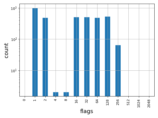

See also

SAMFlags for meaning of each flag

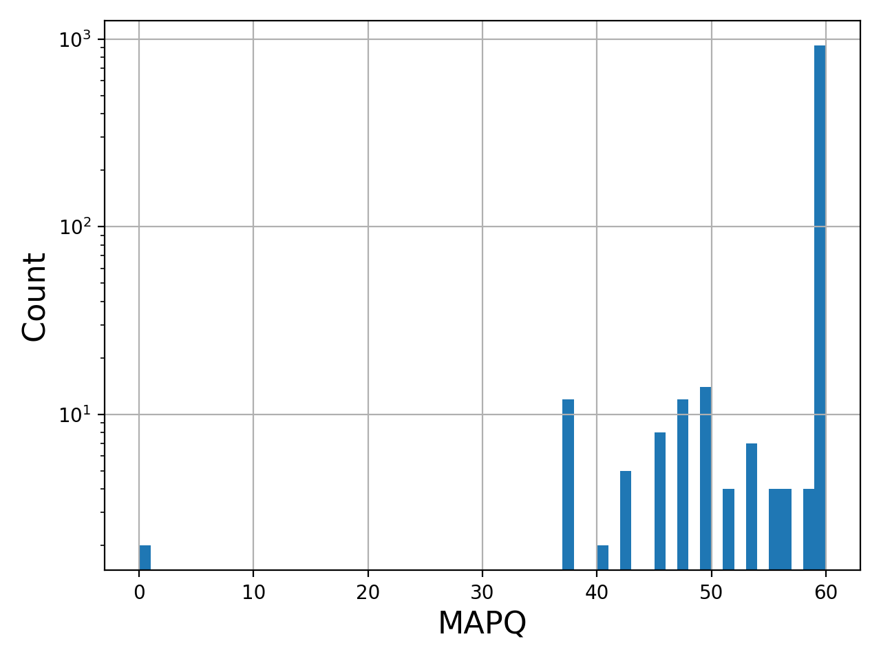
plot_bar_mapq(fontsize=16, filename=None)[source]#

Plots bar plots of the MAPQ (quality) of alignments

from sequana import BAM, sequana_data
b = BAM(sequana_data('test.bam'))
b.plot_bar_mapq()

(Source code, png, hires.png, pdf)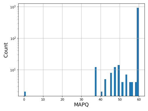

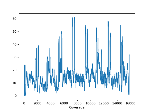
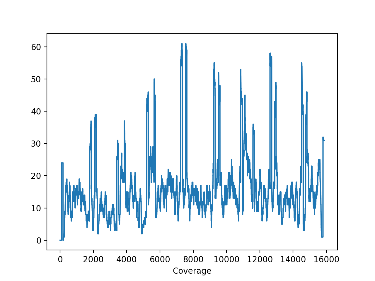
plot_coverage(chrom=None)[source]#

Please use SequanaCoverage for more sophisticated tools to plot the genome coverage

from sequana import sequana_data, BAM
b = BAM(sequana_data("measles.fa.sorted.bam"))
b.plot_coverage()

(Source code, png, hires.png, pdf)

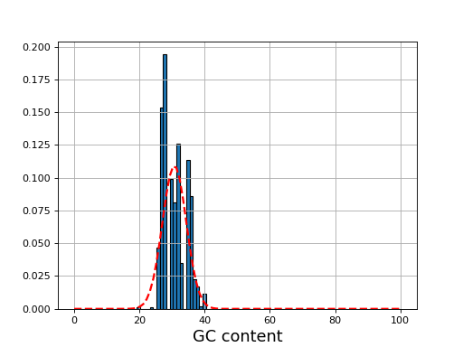
plot_gc_content(fontsize=16, ec='k', bins=100)[source]#

plot GC content histogram

Params bins:: a value for the number of bins or an array (with a copy() method)
Parameters:: ec -- add black contour on the bars

from sequana import BAM, sequana_data
b = BAM(sequana_data('test.bam'))
b.plot_gc_content()

(Source code, png, hires.png, pdf)

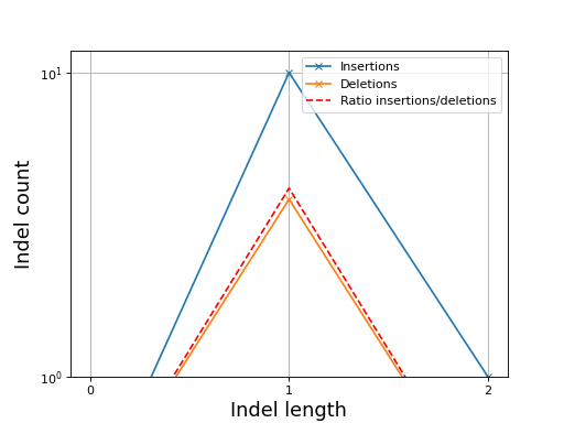
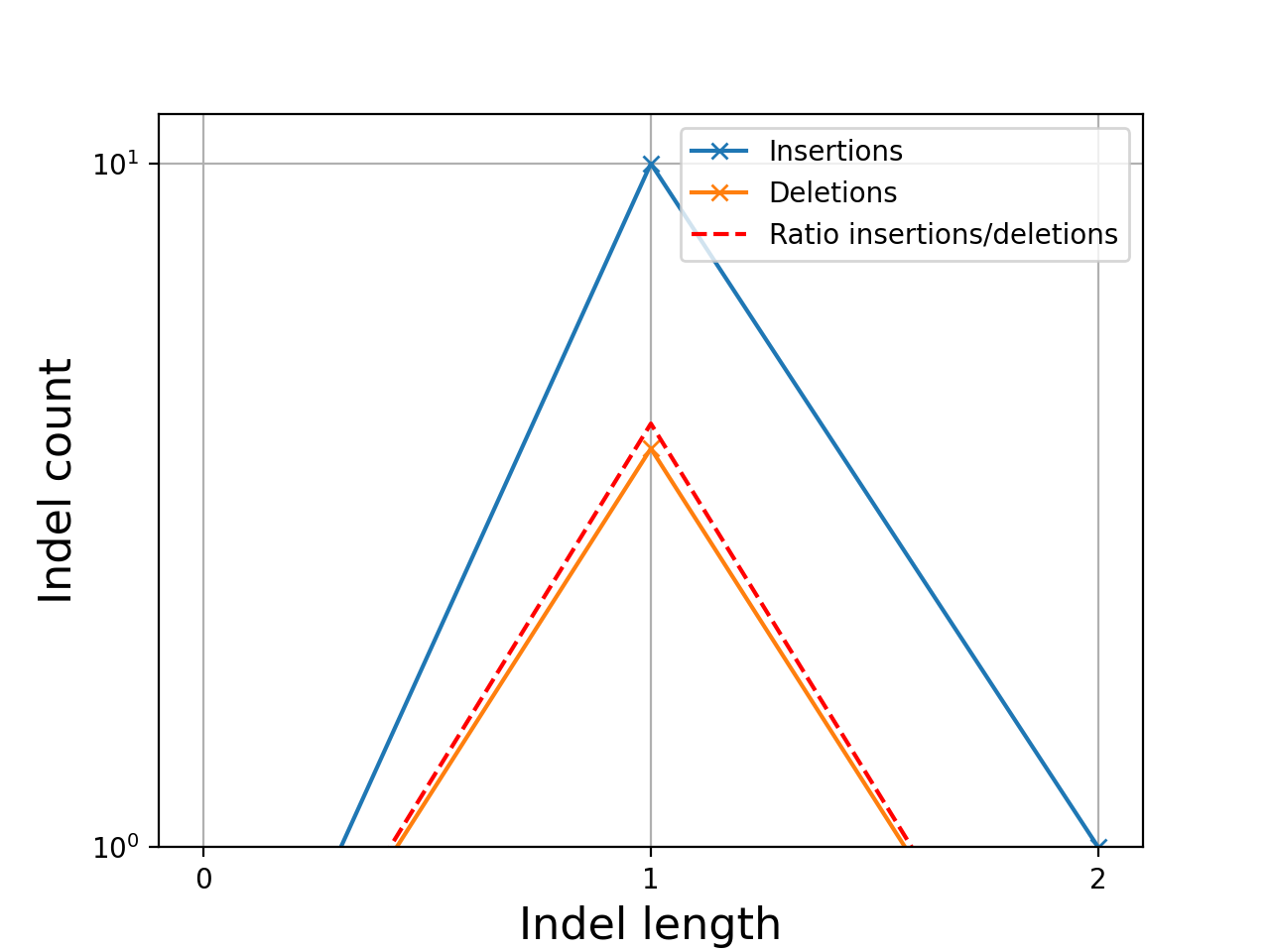
plot_indel_dist(fontsize=16)[source]#

Plot indel count (+ ratio)

Return:: list of insertions, deletions and ratio insertion/deletion for different length starting at 1

from sequana import sequana_data, BAM
b = BAM(sequana_data("measles.fa.sorted.bam"))
b.plot_indel_dist()

(Source code, png, hires.png, pdf)

What you see on this figure is the presence of 10 insertions of length 1, 1 insertion of length 2 and 3 deletions of length 1

# Note that in samtools, several insertions or deletions in a single alignment are ignored and only the first one seems to be reported. For instance 10M1I10M1I stored only 1 insertion in its report; Same comment for deletions.

Todo

speed up and handle long reads cases more effitiently by storing INDELS as histograms rather than lists

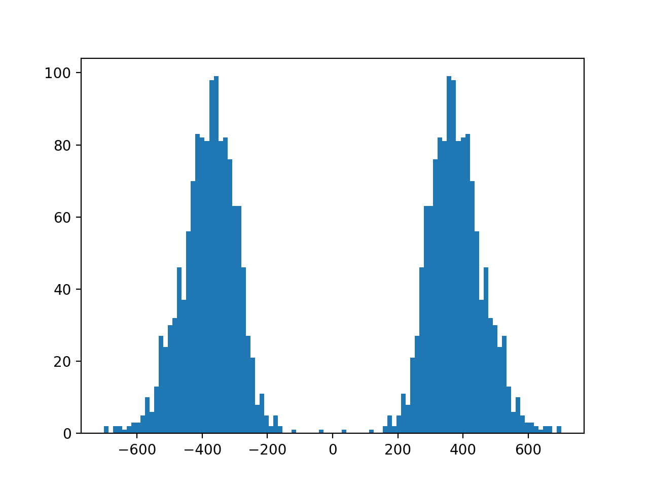
plot_insert_size(max_entries=100000, bins=100, upper_bound=1000, lower_bound=-1000, absolute=False)[source]#

This gives an idea of the insert size without taking into account any intronic gap. The mode should give a good idea of the insert size though.

(Source code, png, hires.png, pdf)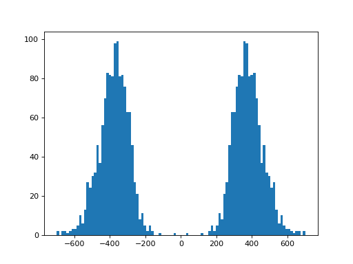

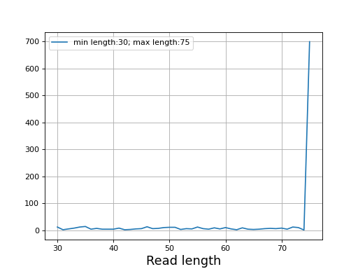
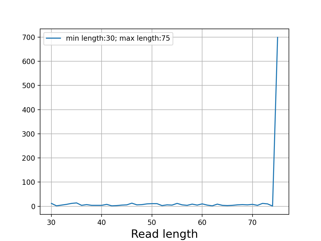
plot_read_length()[source]#

Plot occurences of aligned read lengths

from sequana import sequana_data, BAM
b = BAM(sequana_data("test.bam"))
b.plot_read_length()

(Source code, png, hires.png, pdf)

plotly_hist_read_length(log_y=False, title='', xlabel='Read length (bp)', ylabel='count', **kwargs)[source]#

Histogram of the read length using plotly

Parameters:

log_y
title

any additional arguments is pass to the plotly.express.hist function

reset()[source]#

Close and reopen the underlying alignment file.

This rewinds the read pointer to the very first alignment, which is required before any new iteration over the file. Any previously opened pysam.AlignmentFile is closed before reopening.

property summary#: Count flags/mapq/read length in one pass.

to_fastq(filename)[source]#

Export the BAM to FastQ format

Todo

comments from original reads are not in the BAM so will be missing

Method 1 (bedtools):

bedtools bamtofastq -i JB409847.bam  -fq test1.fastq

Method2 (samtools):

samtools bam2fq JB409847.bam > test2.fastq

Method3 (sequana):

from sequana import BAM
BAM(filename)
BAM.to_fastq("test3.fastq")

Note that the samtools method removes duplicated reads so the output is not identical to method 1 or 3.

to_paf()[source]#

Convert the first alignments that start before position 10 to PAF format.

PAF (Pairwise mApping Format) is a tab-separated text format used by minimap2 and related tools. This method is experimental and currently only exports alignments whose reference_start is less than 10.

Returns:: DataFrame with PAF columns r_name, r_start, r_end, strand, flag, mapq, cigar, q_name, q_len, q_start, and q_end.
Return type:: pandas.DataFrame

class SAMFlags(value=4095)[source]#

Utility to extract bits from a SAM flag

>>> from sequana import SAMFlags
>>> sf = SAMFlags(257)
>>> sf.get_flags()
[1, 256]

You can also print the bits and their description:

print(sf)

bit	Meaning/description
0	mapped segment
1	template having multiple segments in sequencing
2	each segment properly aligned according to the aligner
4	segment unmapped
8	next segment in the template unmapped
16	SEQ being reverse complemented
32	SEQ of the next segment in the template being reverse complemented
64	the first segment in the template
128	the last segment in the template
256	secondary alignment
512	not passing filters, such as platform/vendor quality controls
1024	PCR or optical duplicate
2048	supplementary alignment

Reference:: http://samtools.github.io/hts-specs/SAMv1.pdf

Initialise a SAMFlags helper.

Parameters:: value (int) -- integer SAM flag value. Defaults to 4095 (all bits set).

get_flags()[source]#: Return the individual bits included in the flag

get_meaning()[source]#: Return all description sorted by bit

Coverage #

class Coverage(N=None, L=None, G=None, a=None)[source]#

Utilities related to Lander and Waterman theory

We denote $G$ the genome length in nucleotides and $L$ the read length in nucleotides. These two numbers are in principle well defined since $G$ is defined by biology and $L$ by the sequencing machine.

The total number of reads sequenced during an experiment is denoted $N$ . Therefore the total number of nucleotides is simply $NL$ .

The depth of coverage (DOC) at a given nucleotide position is the number of times that a nucleotide is covered by a mapped read.

The theoretical fold-coverage is defined as :

$a = NL/G$

that is the average number of times each nucleotide is expected to be sequenced (in the whole genome). The fold-coverage is often denoted $aX$ (e.g., 50X).

In the Coverage class, $G$ and $N$ are fixed at the beginning. Then, if one changes $a$ , then $N$ is updated and vice-versa so that the relation $a=NL/G$ is always true:

>>> cover = Coverage(G=1000000, L=100)
>>> cover.N = 100000    # number of reads
>>> cover.a             # What is the mean coverage
10
>>> cover.a = 50
>>> cover.N
500000

From the equation aforementionned, and assuming the reads are uniformly distributed, we can answer a few interesting questions using probabilities.

In each chromosome, a read of length $L$ could start at any position (except the last position L-1). So in a genome $G$ with $n_c$ chromosomes, there are $G - n_c (L-1)$ possible starting positions. In general $G >> n_c (L-1)$ so the probability that one of the $N$ read starts at any specific nucleotide is $N/G$ .

The probability that a read (of length $L$ ) covers a given position is $L/G$ . The probability of not covering that location is $1-L/G$ . For $N$ fragments, we obtain the probability $\left(1-L/G\right)^N$ . So, the probability of covering a given location with at least one read is :

$P = 1 - \left(1- \frac{L}{G}\right)^N$

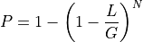
Since in general, N>>1, we have:

$P = 1- \exp^{-NL/G}$

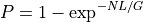
From this equation, we can derive the fold-coverage required to have e.g., $E=99\%$ of the genome covered:

$a = log(-1/(E-1)$

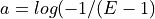
equivalent to

$a = -log(1-E)$

The method get_required_coverage() uses this equation. However, for numerical reason, one should not provide $E$ as an argument but (1-E). See get_required_coverage()

Other information can also be derived using the methods get_mean_number_contigs(), get_mean_contig_length(), get_mean_contig_length().

See also

get_table() that provides a summary of all these quantities for a range of coverage.

Reference:: http://www.math.ucsd.edu/~gptesler/283/FA14/slides/shotgun_14-handout.pdf

property G#: genome length

property L#: length of the reads

property N#: number of reads defined as aG/L

property a#: coverage defined as NL/G

get_mean_contig_length()[source]#: Expected length of the contigs

$\frac{e^a-1)L}{a}$

get_mean_number_contigs()[source]#

Expected number of contigs

A binomial distribution with parameters $N$ and $p$

$\left(\frac{aG}{L}\right) \exp^{-a}$

get_mean_reads_per_contig()[source]#

Expected number of reads per contig

Number of reads divided by expected number of contigs:

$N / (N\exp^{-a}) = e^a$

get_percent_genome_sequenced()[source]#: Return percent of the genome covered

$100 (1-\exp{-a})$

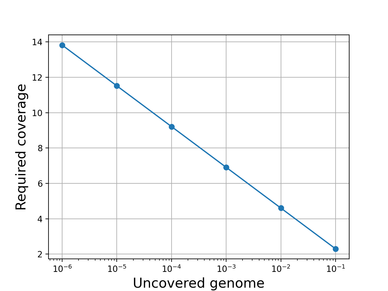
get_required_coverage(M=0.01)[source]#

Return the required coverage to ensure the genome is covered

A general question is what should be the coverage to make sure that e.g. E=99% of the genome is covered by at least a read.

The answer is:

$\log^{-1/(E-1)}$

This equation is correct but have a limitation due to floating precision. If one provides E=0.99, the answer is 4.6 but we are limited to a maximum coverage of about 36 when one provides E=0.9999999999999999 after which E is rounded to 1 on most computers. Besides, it is no convenient to enter all those numbers. A scientific notation would be better but requires to work with $M=1-E$ instead of $E$ .

$\log^{-1/ - M}$

So instead of asking the question what is the requested fold coverage to have 99% of the genome covered, we ask the question what is the requested fold coverage to have 1% of the genome not covered. This allows us to use $M$ values as low as 1e-300 that is a fold coverage as high as 690.

Parameters:: M (float) -- this is the fraction of the genome not covered by any reads (e.g. 0.01 for 1%). See note above.
Returns:: the required fold coverage

(Source code, png, hires.png, pdf)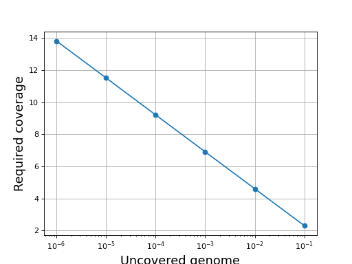

The inverse equation is required fold coverage = [log(-1/(E - 1))]

get_summary()[source]#: Return a summary (dictionary) for the current fold coverage a

get_table(coverage=None)[source]#

Return a summary dataframe for a set of fold coverage

Parameters:: coverage (list) -- if None, coverage list starts at 0.5 and ends at 10 with a step of 0.5

Utilities for the genome coverage

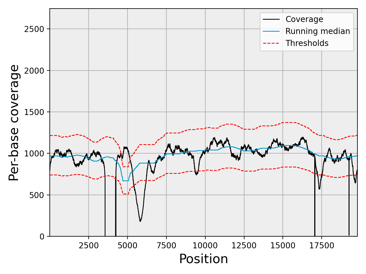
class ChromosomeCov(genomecov, chrom_name, thresholds=None, chunksize=5000000)[source]#

Factory to manipulate coverage and extract region of interests.

Example:

from sequana import SequanaCoverage, sequana_data
filename = sequana_data("virus.bed")

gencov = SequanaCoverage(filename)

chrcov = gencov[0]
chrcov.running_median(n=3001)
chrcov.compute_zscore()
chrcov.plot_coverage()

df = chrcov.get_rois().get_high_rois()

(Source code, png, hires.png, pdf)

The df variable contains a dataframe with high region of interests (over covered)

If the data is large, the input data set is split into chunk. See chunksize, which is 5,000,000 by default.

If your data is larger, then you should use the run() method.

See also

sequana_coverage standalone application

constructor

Parameters:

df -- dataframe with position for a chromosome used within SequanaCoverage. Must contain the following columns: ["pos", "cov"]
genomecov
chrom_name -- to save space, no need to store the chrom name in the dataframe.
thresholds -- a data structure DoubleThresholds that holds the double threshold values.
chunksize -- if the data is large, it is split and analysed by chunk. In such situations, you should use the run() instead of calling the running_median and compute_zscore functions.

property BOC#: breadth of coverage

property C3#

property C4#

property CV#: The coefficient of variation (CV) is defined as sigma / mu

property DOC#: depth of coverage

property STD#: standard deviation of depth of coverage

property bed#

compute_zscore(k=2, use_em=True, clip=4, verbose=True, force_models=None)[source]#

Compute zscore of coverage and normalized coverage.

Parameters:

k (int) -- Number gaussian predicted in mixture (default = 2)
use_em -- use Expectation-Maximization (EM) algorithm
clip (float) -- ignore values above the clip threshold
force_models (bool) -- if set, fitted models is ignored and replaced with 2 Gaussian models where the main model has mean of 1 and represent 90% of the data. Useful to override normal behavior

Store the results in the df attribute (dataframe) with a column named zscore.

Note

needs to call running_median() before hand.

property df#

property evenness#

Return Evenness of the coverage

Reference:: Konrad Oexle, Journal of Human Genetics 2016, Evaulation of the evenness score in NGS.

work before or after normalisation but lead to different results.

get_centralness(threshold=3)[source]#

Proportion of central (normal) genome coverage

This is 1 - (number of non normal data) / (total length)

Note

depends on the thresholds attribute being used.

Note

depends slightly on $W$ the running median window

get_gaussians()[source]#

get_gc_correlation()[source]#

Return the correlation between the coverage and GC content

The GC content is the one computed in SequanaCoverage.compute_gc_content() (default window size is 101)

get_rois()[source]#

Keep positions with zscore outside of the thresholds range.

Returns:: a dataframe from FilteredGenomeCov

Note

depends on the thresholds low and high values.

get_stats()[source]#

Return basic stats about the coverage data

only "cov" column is required.

Returns:: dictionary

get_summary(C3=None, C4=None, stats=None, caller='sequana.bedtools')[source]#

init()[source]#

moving_average(n, circular=False)[source]#

Compute moving average of the genome coverage

Parameters:

n -- window's size. Must be odd
circular (bool) -- is the chromosome circular or not

Store the results in the df attribute (dataframe) with a column named ma.

next()[source]#

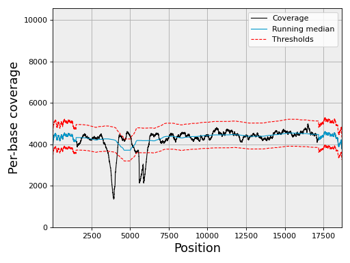
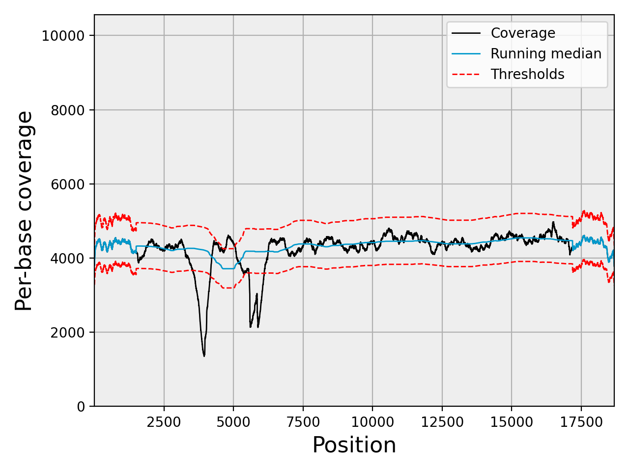
plot_coverage(filename=None, fontsize=16, rm_lw=1, rm_color='#0099cc', rm_label='Running median', th_lw=1, th_color='r', th_ls='--', main_color='k', main_lw=1, main_kwargs={}, sample=True, set_ylimits=True, x1=None, x2=None, clf=True)[source]#

Plot coverage as a function of base position.

Parameters:

filename
rm_lw -- line width of the running median
rm_color -- line color of the running median
rm_color -- label for the running median
th_lw -- line width of the thresholds
th_color -- line color of the thresholds
main_color -- line color of the coverage
main_lw -- line width of the coverage
sample -- if there are more than 1 000 000 points, we use an integer step to skip data points. We can still plot all points at your own risk by setting this option to False
set_ylimits -- we want to focus on the "normal" coverage ignoring unsual excess. To do so, we set the yaxis range between 0 and a maximum value. This maximum value is set to the minimum between the 10 times the mean coverage and 1.5 the maximum of the high coverage threshold curve. If you want to let the ylimits free, set this argument to False
x1 -- restrict lower x value to x1
x2 -- restrict lower x value to x2 (x2 must be greater than x1)

Note

if there are more than 1,000,000 points, we show only 1,000,000 by points. For instance for 5,000,000 points,

In addition to the coverage, the running median and coverage confidence corresponding to the lower and upper zscore thresholds are shown.

Note

uses the thresholds attribute.

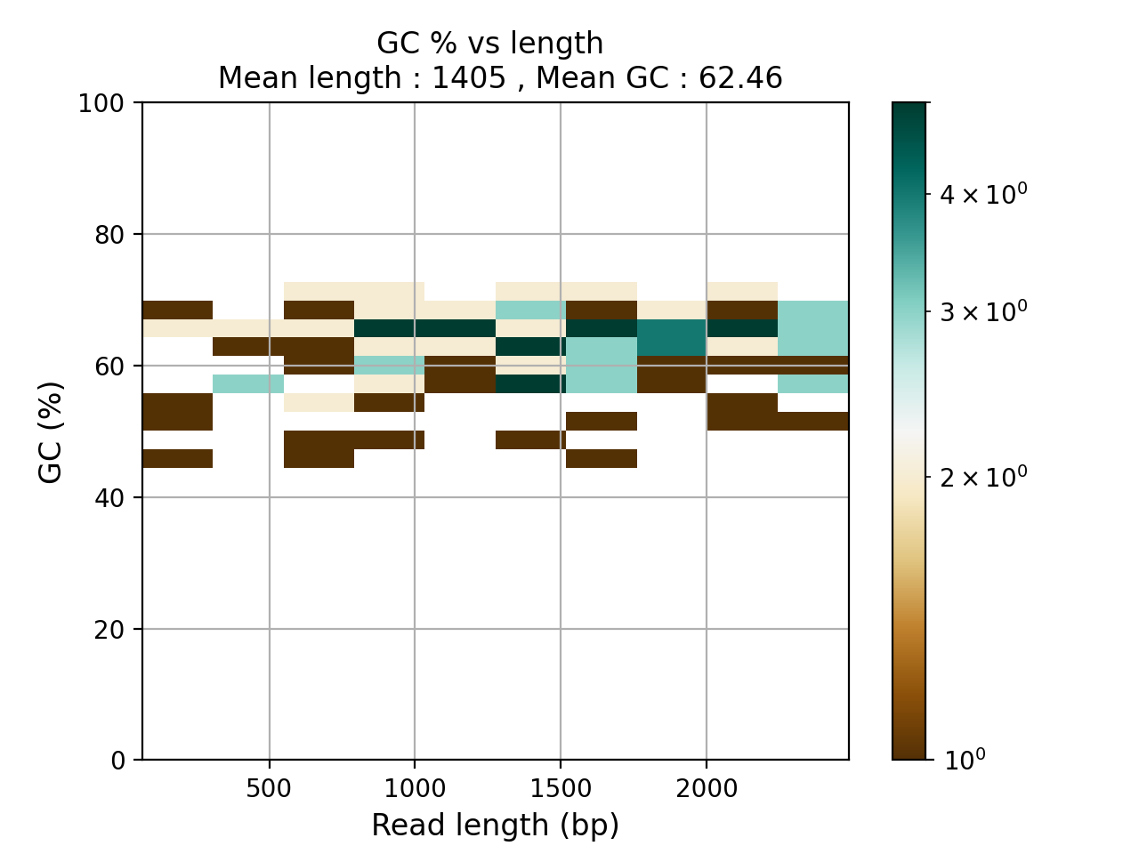
plot_gc_vs_coverage(filename=None, bins=None, Nlevels=None, fontsize=20, norm='log', ymin=0, ymax=100, contour=True, cmap='BrBG', **kwargs)[source]#: Plot histogram 2D of the GC content versus coverage

plot_hist_coverage(logx=True, logy=True, fontsize=16, N=25, fignum=1, hold=False, alpha=0.8, ec='k', filename=None, zorder=10, **kw_hist)[source]#

Parameters:

plot_hist_normalized_coverage(filename=None, binwidth=0.05, max_z=3)[source]#: Barplot of the normalized coverage with gaussian fitting

plot_hist_zscore(fontsize=16, filename=None, max_z=6, binwidth=0.5, **hist_kargs)[source]#: Barplot of the zscore values

plot_rois(x1, x2, set_ylimits=False, rois=None, fontsize=16, color_high='r', color_low='g', clf=True)[source]#

property rois#

run(W, k=2, circular=False, binning=None, cnv_delta=None)[source]#

running_median(n, circular=False)[source]#

Compute running median of genome coverage

Parameters:

n (int) -- window's size.
circular (bool) -- if a mapping is circular (e.g. bacteria whole genome sequencing), set to True

Store the results in the df attribute (dataframe) with a column named rm.

Changed in version 0.1.21: Use Pandas rolling function to speed up computation.

to_csv(filename=None, start=None, stop=None, **kwargs)[source]#

Write CSV file of the dataframe.

Parameters:

filename (str) -- csv output filename. If None, return string.
start (int) -- start row index.
stop (int) -- stop row index.

Params of pandas.DataFrame.to_csv():

Parameters:

columns (list) -- columns you want to write.
header (bool) -- determine if the header is written.
index (bool) -- determine if the index is written.
float_format (str) -- determine the float format.

class DoubleThresholds(low=-3, high=3, ldtr=0.5, hdtr=0.5)[source]#

Simple structure to handle the double threshold for negative and positive sides

Used by the SequanaCoverage and related classes.

dt = DoubleThresholds(-3, 4, 0.5, 0.5)

This means the low threshold is -3 while the high threshold is 4. The two following values must be between 0 and 1 and are used to define the value of the double threshold set to half the value of the main threshold.

Internally, the main thresholds are stored in the low and high attributes. The secondary thresholds are derived from the main thresholds and the two ratios. The ratios are named ldtr and hdtr for low double threshold ratio and high double threshold ratio. The secondary thresholds are denoted low2 and high2 and are update automatically if low, high, ldtr or hdtr are changed.

copy()[source]#

get_args()[source]#

property hdtr#

property high#

property high2#

property ldtr#

property low#

property low2#

class SequanaCoverage(input_filename, annotation_file=None, low_threshold=-4, high_threshold=4, ldtr=0.5, hdtr=0.5, force=False, chunksize=5000000, quiet_progress=False, chromosome_list=[], reference_file=None, gc_window_size=101)[source]#

Create a list of dataframe to hold data from a BED file generated with samtools depth.

This class can be used to plot the coverage resulting from a mapping, which is stored in BED format. The BED file may contain several chromosomes. There are handled independently and accessible as a list of ChromosomeCov instances.

Example:

from sequana import SequanaCoverage, sequana_data

filename = sequana_data('JB409847.bed')
reference = sequana_data("JB409847.fasta")

gencov = SequanaCoverage(filename)

# you can change the thresholds:
gencov.thresholds.low = -4
gencov.thresholds.high = 4
#gencov.compute_gc_content(reference)

gencov = SequanaCoverage(filename)
for chrom in gencov:
    chrom.running_median(n=3001, circular=True)
    chrom.compute_zscore()
    chrom.plot_coverage()

(Source code, png, hires.png, pdf)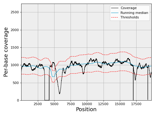

Results are stored in a list of ChromosomeCov named chr_list. For Prokaryotes and small genomes, this API is convenient but takes lots of memory for larger genomes.

Computational time information: scanning 24,000,000 rows

constructor (scanning 40,000,000 rows): 45s

select contig of 24,000,000 rows: 1min20

running median: 16s

compute zscore: 9s

c.get_rois() ():

constructor

Parameters:

input_filename (str) -- the input data with results of a bedtools genomecov run. This is just a 3-column file. The first column is a string (chromosome), second column is the base postion and third is the coverage.
annotation_file (str) -- annotation file of your reference (GFF3/Genbank).
low_threshold (float) -- threshold used to identify under-covered genomic region of interest (ROI). Must be negative
high_threshold (float) -- threshold used to identify over-covered genomic region of interest (ROI). Must be positive
ldtr (float) -- fraction of the low_threshold to be used to define the intermediate threshold in the double threshold method. Must be between 0 and 1.
rdtr (float) -- fraction of the low_threshold to be used to define the intermediate threshold in the double threshold method. Must be between 0 and 1.
chunksize -- size of segments to analyse. If a chromosome is larger than the chunk size, it is split into N chunks. The segments are analysed indepdently and ROIs and summary joined together. Note that GC, plotting functionalities will only plot the first chunk.
force -- some constraints are set in the code to prevent unwanted memory issues with specific data sets of parameters. Currently, by default, (i) you cannot set the threshold below 2.5 (considered as noise).
chromosome_list -- list of chromosomes to consider (names). This is useful for very large input data files (hundreds million of lines) where each chromosome can be analysed one by one. Used by the sequana_coverage standalone. The only advantage is to speed up the constructor creation and could also be used by the Snakemake implementation.
reference_file -- if provided, computes the GC content
gc_window_size (int) -- size of the GC sliding window. (default 101)

property annotation_file#: Get or set the genbank filename to annotate ROI detected with ChromosomeCov.get_roi(). Changing the genbank filename will configure the SequanaCoverage.feature_dict.

property circular#: Get the circularity of chromosome(s). It must be a boolean.

property feature_dict#: Get the features dictionary of the genbank.

property gc_window_size#: Get or set the window size to compute the GC content.

get_stats()[source]#

Return basic statistics for each chromosome

Returns:: dictionary with chromosome names as keys and statistics as values.

See also

ChromosomeCov.

Note

used in sequana_summary standalone

property input_filename#

property reference_file#

property window_size#: Get or set the window size to compute the running median. Size must be an interger.

Data analysis tool

RunningMedian(data, width[, container])

Running median (fast)

class RunningMedian(data, width, container=<class 'list'>)[source]#

Running median (fast)

This is an efficient implementation of running median, faster than SciPy implementation v0.17 and a skip list method.

The main idea comes from a recipe posted in this website: http://code.activestate.com/recipes/576930/#c3 that uses a simple list as proposed in https://gist.github.com/f0k/2f8402e4dfb6974bfcf1 and was adapted to our needs included object oriented implementation.

Note

a circular running median is implemented in sequana.bedtools.SequanaCoverage

from sequana.running_median import RunningMedian
rm = RunningMedian(data, 101)
results = rm.run()

Warning

the first W/2 and last W/2 positions should be ignored since they do not use W values. In this implementation, the last W/2 values are currently set to zero.

This shows how the results agree with scipy

from pylab import *
import scipy.signal
from sequana.running_median import RunningMedian

clf()
x = randn(100)
plot(x, 'k')
plot(RunningMedian(x,9).run(), 'r', lw=4)
plot(scipy.signal.medfilt(x, 9), 'go')
grid()

(Source code, png, hires.png, pdf)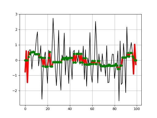

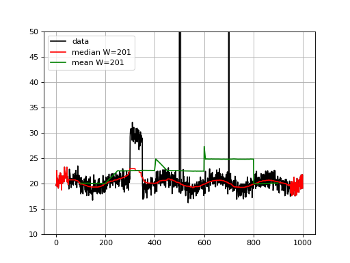
from sequana.running_median import RunningMedian
from pylab import *

N = 1000
X = linspace(0, N-1, N)

# Create some interesting data with SNP and longer over
# represented section.
data = 20 + randn(N) + sin(X*2*pi/1000.*5)
data[300:350] += 10
data[500:505] += 100
data[700] = 1000

plot(X, data, "k", label="data")
rm = RunningMedian(data, 101)
plot(X, rm.run(), 'r', label="median W=201")

from sequana.stats import moving_average as ma
plot(X[100:-100], ma(data, 201), 'g', label="mean W=201")
grid()
legend()
ylim([10, 50])

(Source code, png, hires.png, pdf)

Note that for visualisation, we set the ylimits to 50 but the data at position 500 goes up to 120 and there is an large outlier (1000) at position 700 .

We see that the median is less sensible to the outliers, as expected. The median is highly interesting for large outliers on short duration (e.g. here the peak at position 500) but is also less biases by larger regions.

Note

The beginning and end of the running median are irrelevant. There are actually equal to the data in our implementation.

Note

using blist instead of list is not always faster. It depends on the width of the window being used. list and blist are equivaltn for W below 20,000 (list is slightly faster). However, for large W, blist has an O(log(n)) complexity while list has a O(n) complexity

constructor

Parameters:

data -- your data vector
width -- running window length
container -- a container (defaults to list). Could be a B-tree blist from the blist package but is 30% slower than a pure list for W < 20,000

scipy in O(n) list in sqrt(n) blist in O(log(n))

run()[source]#

running_median(data, width, container=<class 'list'>)[source]#

Assembly and contigs #

class BUSCO(filename='full_table_test.tsv')[source]#

Wrapper of the BUSCO output

"BUSCO provides a quantitative measures for the assessment of a genome assembly, gene set, transcriptome completeness, based on evolutionarily-informed expectations of gene content from near-universal single-copy orthologs selected from OrthoDB v9." -- BUSCO website 2017

This class reads the full report generated by BUSCO and provides some visualisation of this report. The information is stored in a dataframe df. The score can be retrieve with the attribute score in percentage in the range 0-100.

Reference:: http://busco.ezlab.org/

Note

support version 3.0.1 and new formats from v5.X

constructor

Filename:: a valid BUSCO input file (full table). See example in sequana code source (testing)

get_summary_string()[source]#

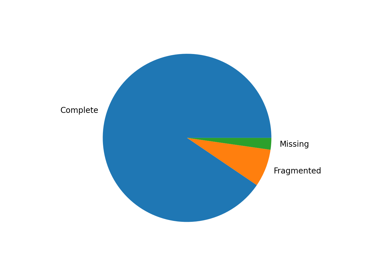
pie_plot(filename=None, hold=False)[source]#

Pie plot of the status (completed / fragment / missed)

from sequana import BUSCO, sequana_data
b = BUSCO(sequana_data("test_busco_full_table.tsv"))
b.pie_plot()

(Source code, png, hires.png, pdf)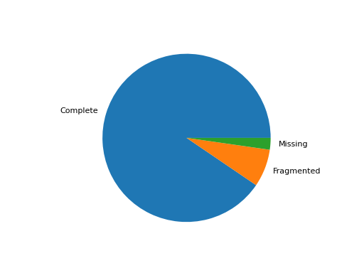

save_core_genomes(contig_file, output_fasta_file='core.fasta')[source]#

Save the core genome based on busco and assembly output

The busco file must have been generated from an input contig file. In the example below, the busco file was obtained from the data.contigs.fasta file:

from sequana import BUSCO
b = BUSCO("busco_full_table.tsv")
b.save_core_genomes("data.contigs.fasta", "core.fasta")

If a gene from the core genome is missing, the extracted gene is made of 100 N's If a gene is duplicated, only the best entry (based on the score) is kept.

If there are 130 genes in the core genomes, the output will be a multi-sequence FASTA file made of 130 sequences.

scatter_plot(filename=None, hold=False)[source]#

Scatter plot of the score versus length of each ortholog

from sequana import BUSCO, sequana_data
b = BUSCO(sequana_data("test_busco_full_table.tsv"))
b.scatter_plot()

(Source code, png, hires.png, pdf)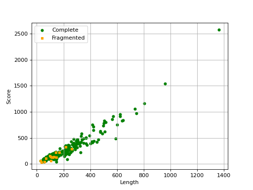

Missing are not show since there is no information about contig .

property score#

summary()[source]#: Return summary information of the missing, completed, fragemented orthologs

class Contigs(filename, mode='canu')[source]#

Utilities for summarising or plotting contig information

Depending on how the FastA file was created, different types of plots can be are available. For instance, if the FastA was created with Canu, nreads and covStat information can be extracted. Therefore, plots such as plot_scatter_contig_length_vs_nreads_cov() and plot_contig_length_vs_nreads() can be used.

Constructor

Parameters:

filename -- input FastA file
canu -- tool that created the output file.

property df#

hist_plot_contig_length(bins=40, fontsize=16, lw=1)[source]#

Plot distribution of contig lengths

Parameters:

bin -- number of bins for the histogram
fontsize -- fontsize for xy-labels
lw -- width of bar contour edges
ec -- color of bar contours

(Source code, png, hires.png, pdf)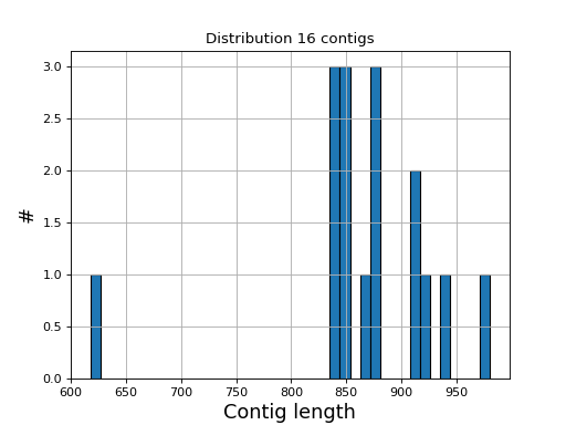

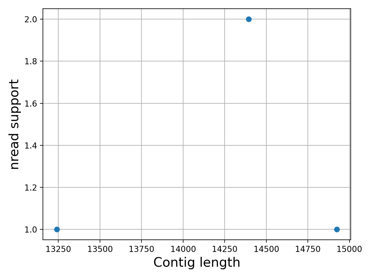
plot_contig_length_vs_nreads(fontsize=16, min_length=5000, min_nread=10, grid=True, logx=True, logy=True)[source]#

Plot contig length versus nreads

In canu, contigs have the number of reads that support them. Here, we can see whether contigs have lots of reads supported them or not.

Note

For Canu output only

(Source code, png, hires.png, pdf)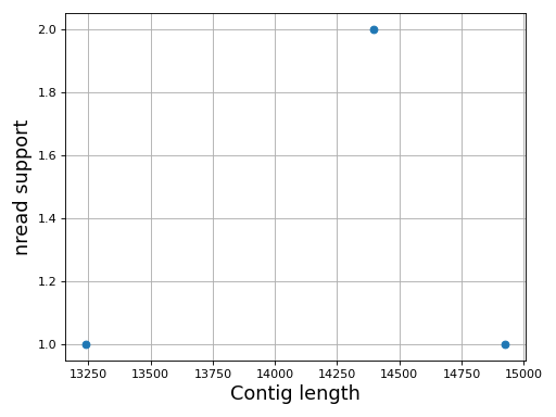

plot_scatter_contig_length_vs_nreads_cov(fontsize=16, vmin=0, vmax=50, min_nreads=20, min_length=5000, grid=True, logx=True, logy=True)[source]#

Scatter plot showing number of support reads and contig lengths

Note

only for Canu output.

(Source code)

stats()[source]#: Return N50, L50 and total cumulated length

class ContigsBase(filename)[source]#

Parent class for contigs data

Constructor

Parameters:: filename -- input file name

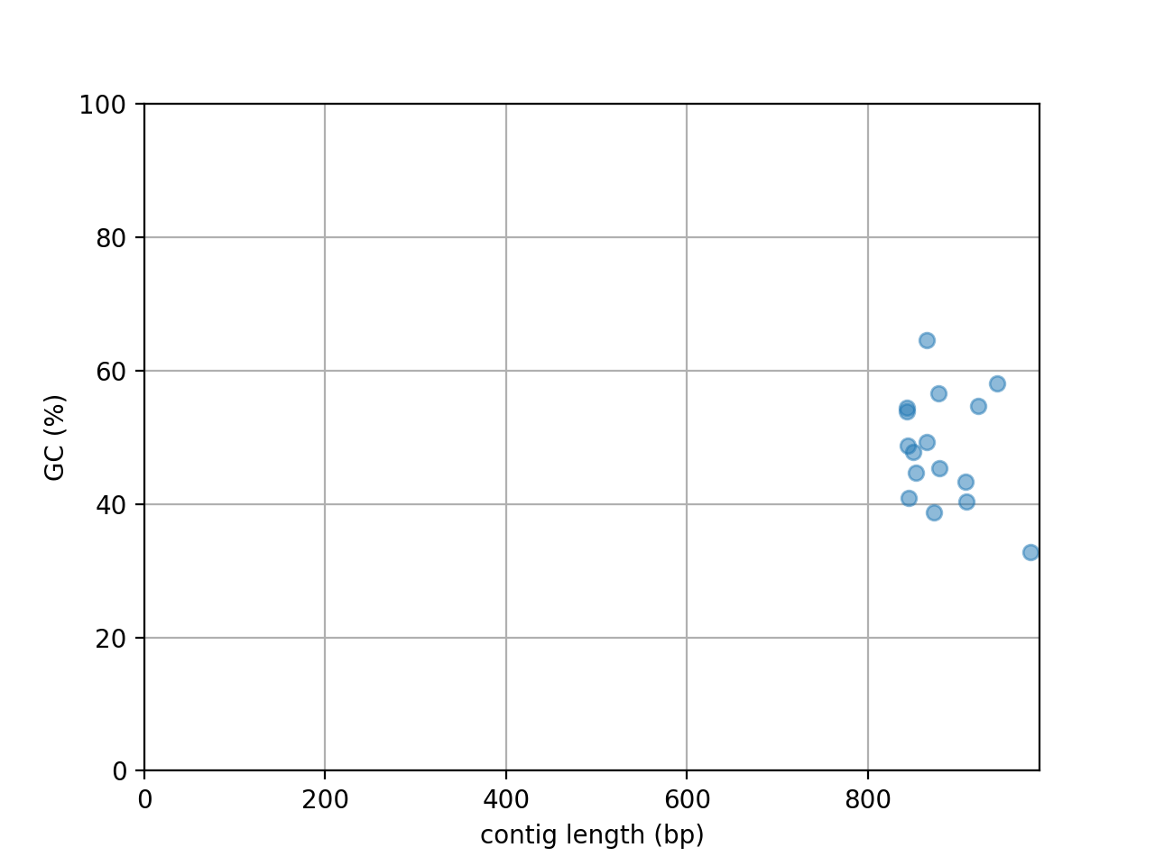
get_gc(window=100)[source]#: Return GC content for each contig

plot_contig_length_vs_GC(alpha=0.5)[source]#

Plot contig GC content versus contig length

(Source code, png, hires.png, pdf)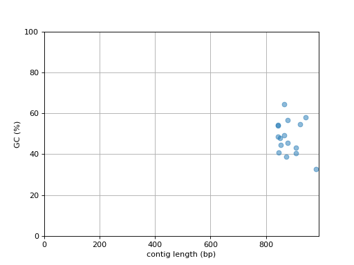

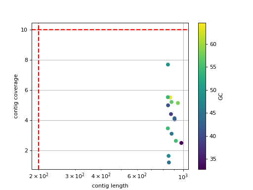
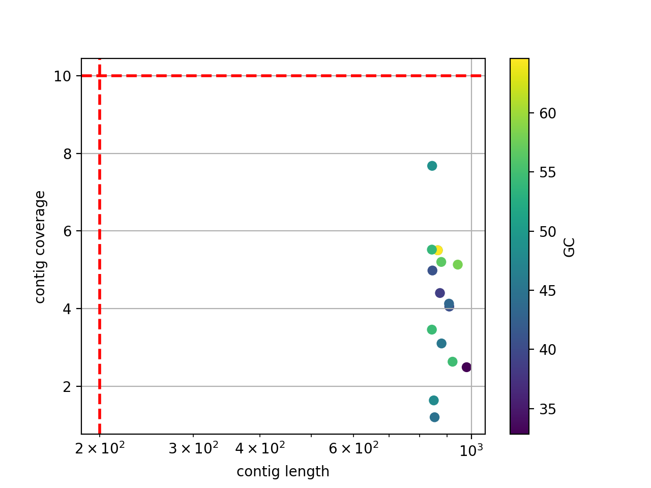
scatter_length_cov_gc(min_length=200, min_cov=10, grid=True, logy=False, logx=True)[source]#

Plot scatter length versus GC content

Parameters:

min_length -- add vertical line to indicate possible contig length cutoff
min_cov -- add horizontal line to indicate possible coverage contig cutff
grid -- add grid to the plot
logy -- set y-axis log scale
logx -- set x-axis log scale

(Source code, png, hires.png, pdf)

class CheckM(filename)[source]#

class MultiCheckM(filenames)[source]#

class CanuScanner(path='.')[source]#

Scan a Canu assembly output directory and collect statistics.

Parses Canu's correction, trimming and assembly stage files to expose read length distributions, k-mer histograms and overlap/correction summaries through helper methods.

Initialise the scanner.

Parameters:: path (str) -- path to the root of a Canu output directory.

getfile(filename)[source]#

hist_read_length(bins=100, fontsize=16)[source]#

Plot the read length histogram for the correction stage.

Parameters:

bins (int) -- number of bins for the histogram.
fontsize (int) -- axis label font size.

Returns:

pandas DataFrame with the parsed read information.

hist_read_length2(fontsize=16)[source]#

hist_trimming_read_length(bins=100, fontsize=16)[source]#

Plot the read length histogram for the trimming stage.

Parameters:

bins (int) -- number of bins for the histogram.
fontsize (int) -- axis label font size.

Returns:

pandas DataFrame with the parsed read information.

plot_correction_check1(alpha=0.5)[source]#

plot_kmer(bins=100)[source]#

scan_correction()[source]#: Read the correction load.dat file and populate the data dictionary with kept and skipped reads (number of reads and base pairs).

scan_trimming()[source]#

set_overlap_filtering()[source]#

set_read_correction()[source]#

Taxonomy #

class KrakenAnalysis(fastq, database, threads=4, confidence=0)[source]#

Run kraken on a set of FastQ files

In order to run a Kraken analysis, we firtst need a local database. We provide a Toy example. The ToyDB is downloadable as follows ( you will need to run the following code only once):

from sequana import KrakenDownload
kd = KrakenDownload()
kd.download_kraken_toydb()

See also

KrakenDownload for more databases

The path to the database is required to run the analysis. It has been stored in the directory ./config/sequana/kraken_toydb under Linux platforms The following code should be platform independent:

import os
from sequana import sequana_config_path
database = sequana_config_path + os.sep + "kraken_toydb")

Finally, we can run the analysis on the toy data set:

from sequana import sequana_data
data = sequana_data("Hm2_GTGAAA_L005_R1_001.fastq.gz", "data")
ka = KrakenAnalysis(data, database=database)
ka.run()

This creates a file named kraken.out. It can be interpreted with KrakenResults

Constructor

Parameters:

fastq -- either a fastq filename or a list of 2 fastq filenames
database -- the path to a valid Kraken database
threads -- number of threads to be used by Kraken
confidence -- parameter used by kraken2
return

run(output_filename=None, output_filename_classified=None, output_filename_unclassified=None, only_classified_output=False)[source]#

Performs the kraken analysis

Parameters:

output_filename (str) -- if not provided, a temporary file is used and stored in kraken_output.
output_filename_classified (str) -- not compressed
output_filename_unclassified (str) -- not compressed

class KrakenDB(filename)[source]#

Class to handle a kraken DB

property version#

class KrakenPipeline(fastq, database, threads=4, output_directory='kraken', dbname=None, confidence=0)[source]#

Used by the standalone application sequana_taxonomy

This runs Kraken on a set of FastQ files, transform the results in a format compatible for Krona, and creates a Krona HTML report.

from sequana import KrakenPipeline
kt = KrakenPipeline(["R1.fastq.gz", "R2.fastq.gz"], database="krakendb")
kt.run()
kt.show()

Sequana project provides pre-compiled Kraken databases on zenodo. Please, use the sequana_taxonomy standalone to download them. Under Linux, they are stored in ~/.config/sequana/kraken2_dbs

Constructor

Parameters:

fastq -- either a fastq filename or a list of 2 fastq filenames
database -- the path to a valid Kraken database
threads -- number of threads to be used by Kraken
output_directory -- output filename of the Krona HTML page
dbname

Description: internally, once Kraken has performed an analysis, reads are associated to a taxon (or not). We then find the correponding lineage and scientific names to be stored within a Krona formatted file. KtImportTex is then used to create the Krona page.

run(output_filename_classified=None, output_filename_unclassified=None, only_classified_output=False)[source]#: Run the analysis using Kraken and create the Krona output

class KrakenResults(filename='kraken.out', verbose=True, mode='ncbi')[source]#

Translate Kraken results into a Krona-compatible file

If you run a kraken analysis with KrakenAnalysis, you will end up with a file e.g. named kraken.out (by default).

You could use kraken-translate but then you need extra parsing to convert into a Krona-compatible file. Here, we take the output from kraken and directly transform it to a krona-compatible file.

kraken2 uses the --use-names that needs extra parsing.

k = KrakenResults("kraken.out")
k.kraken_to_krona()

Then format expected looks like:

C    HISEQ:426:C5T65ACXX:5:2301:18719:16377    1    203    1:71 A:31 1:71
C    HISEQ:426:C5T65ACXX:5:2301:21238:16397    1    202    1:71 A:31 1:71

Where each row corresponds to one read.

"562:13 561:4 A:31 0:1 562:3" would indicate that:

the first 13 k-mers mapped to taxonomy ID #562
the next 4 k-mers mapped to taxonomy ID #561
the next 31 k-mers contained an ambiguous nucleotide
the next k-mer was not in the database
the last 3 k-mers mapped to taxonomy ID #562

For kraken2, format is slighlty different since it depends on paired or not. If paired,

C   read1 2697049 151|151 2697049:117 |:| 0:1 2697049:116

See kraken documentation for details.

Note

a taxon of ID 1 (root) means that the read is classified but in differen domain. DerrickWood/kraken#100

Note

This takes care of fetching taxons and the corresponding lineages from online web services.

constructor

Parameters:: filename -- the input from KrakenAnalysis class

boxplot_classified_vs_read_length()[source]#: Show distribution of the read length grouped by classified or not

property df#

get_taxonomy_db(ids)[source]#

Retrieve taxons given a list of taxons

Parameters:: ids (list) -- list of taxons as strings or integers. Could also be a single string or a single integer
Returns:: a dataframe

Note

the first call first loads all taxons in memory and takes a few seconds but subsequent calls are much faster

histo_classified_vs_read_length()[source]#: Show distribution of the read length grouped by classified or not

kraken_to_csv(filename, dbname)[source]#

kraken_to_json(filename, dbname)[source]#

kraken_to_krona(output_filename=None, nofile=False)[source]#

Returns:: status: True is everything went fine otherwise False

plot(kind='pie', cmap='tab20c', threshold=1, radius=0.9, textcolor='red', delete_krona_file=False, **kargs)[source]#

A simple non-interactive plot of taxons

Returns:: None if no taxon were found and a dataframe otherwise

A Krona Javascript output is also available in kraken_to_krona()

from sequana import KrakenResults, sequana_data
test_file = sequana_data("kraken.out")
k = KrakenResults(test_file)
df = k.plot(kind='pie')

(Source code, png, hires.png, pdf)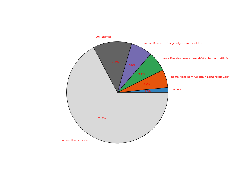

See also

to generate the data see KrakenPipeline or the standalone application sequana_taxonomy.

Todo

For a future release, we could use this kind of plot https://stackoverflow.com/questions/57720935/how-to-use-correct-cmap-colors-in-nested-pie-chart-in-matplotlib

plot2(kind='pie', fontsize=12)[source]#: This is the simplified static krona-like plot included in HTML reports

property taxons#

to_js(output='krona.html')[source]#

class KrakenConsensus(filename_fastq, fof_databases, threads=1, output_directory='./kraken_sequential/', keep_temp_files=False, output_filename_unclassified=None, output_filename_classified=None, force=False, confidence=0)[source]#

Kraken Sequential Analysis

This runs Kraken on a FastQ file with multiple k-mer databases in a sequencial way way. Unclassified sequences with the first database are input for the second, and so on.

The input may be a single FastQ file or paired, gzipped or not. FastA are also accepted.

constructor

Parameters:

filename_fastq -- FastQ file to analyse
fof_databases -- file that contains a list of databases paths (one per line). The order is important. Note that you may also provide a list of datab ase paths.
threads -- number of threads to be used by Kraken
output_directory -- name of the output directory
keep_temp_files -- bool, if True, will keep intermediate files from each Kraken analysis, and save html report at each step
force (bool) -- if the output directory already exists, the instanciation fails so that the existing data is not overrwritten. If you wish to overwrite the existing directory, set this parameter to iTrue.

run(dbname='multiple', output_prefix='kraken_final')[source]#

Run the sequential analysis

Parameters:

dbname
output_prefix

Returns:

dictionary summarizing the databases names and classified/unclassied

This method does not return anything creates a set of files:

kraken_final.out
krona_final.html
kraken.png (pie plot of the classified/unclassified reads)

Note

the databases are run in the order provided in the constructor.

class KrakenDownload(output_dir=None)[source]#

Utility to download Kraken DB and place them in a local directory

from sequana import KrakenDownload
kd = KrakenDownload()
kd.download('toydb')

download(name)[source]#

class MultiKrakenResults(filenames, sample_names=None)[source]#

Select several kraken output and creates summary plots

import glob
mkr = MultiKrakenResults(glob.glob("*/*/kraken.csv"))
mkr.plot_stacked_hist()

get_df(limit=5, rank='kingdom')[source]#

plot_stacked_hist(output_filename=None, dpi=200, kind='barh', fontsize=10, edgecolor='k', lw=1, width=1, ytick_fontsize=10, max_labels=50, max_sample_name_length=30, rank='kingdom')[source]#: Summary plot of reads classified.

class MultiKrakenResults2(filenames, sample_names=None)[source]#

Select several kraken output and creates summary plots

import glob
mkr = MultiKrakenResults2(glob.glob("*/*/summary.json"))
mkr.plot_stacked_hist()

get_df(limit=5, sorting_method='sample_name')[source]#

plot_stacked_hist(output_filename=None, dpi=200, kind='barh', fontsize=10, edgecolor='k', lw=2, width=1, ytick_fontsize=10, max_labels=50, alpha=0.8, colors=None, cmap='viridis', sorting_method='sample_name', max_sample_name_length=30)[source]#

Summary plot of reads classified.

Parameters:

sorting_method -- only by sample name for now
cmap -- a valid matplotlib colormap. viridis is the default sequana colormap.

if you prefer to use a colormap, you can use:

from matplotlib import cm
cm = matplotlib.colormap
colors = [cm.get_cmap(cmap)(x) for x in pylab.linspace(0.2, 1, L)]

class KrakenSequential(filename_fastq, fof_databases, threads=1, output_directory='./kraken_sequential/', keep_temp_files=False, output_filename_unclassified=None, output_filename_classified=None, force=False, confidence=0)[source]#

Kraken Sequential Analysis

This runs Kraken on a FastQ file with multiple k-mer databases in a sequencial way way. Unclassified sequences with the first database are input for the second, and so on.

The input may be a single FastQ file or paired, gzipped or not. FastA are also accepted.

constructor

Parameters:

filename_fastq -- FastQ file to analyse
fof_databases -- file that contains a list of databases paths (one per line). The order is important. Note that you may also provide a list of datab ase paths.
threads -- number of threads to be used by Kraken
output_directory -- name of the output directory
keep_temp_files -- bool, if True, will keep intermediate files from each Kraken analysis, and save html report at each step
force (bool) -- if the output directory already exists, the instanciation fails so that the existing data is not overrwritten. If you wish to overwrite the existing directory, set this parameter to iTrue.

run(dbname='multiple', output_prefix='kraken_final')[source]#

Run the sequential analysis

Parameters:

dbname
output_prefix

Returns:

dictionary summarizing the databases names and classified/unclassied

This method does not return anything creates a set of files:

kraken_final.out
krona_final.html
kraken.png (pie plot of the classified/unclassified reads)

Note

the databases are run in the order provided in the constructor.

class KronaMerger(filename)[source]#

Utility to merge two Krona files

Imagine those two files (formatted for Krona; first column is a counter):

 Bacteria    Proteobacteria  species1
Bacteria    Proteobacteria  species4

Bacteria    Proteobacteria  species3
Bacteria    Proteobacteria  species2
Bacteria    Proteobacteria  species1

You can merge the two files. The first and last lines correspond to the same taxon (species1) so we should end up with a new Krona file with 4 lines only.

The test files are available within Sequana as test_krona_k1.tsv and test_krona_k2.tsv:

from sequana import KronaMerger, sequana_data
k1 = KronaMerger(sequana_data("test_krona_k1.tsv"))
k2 = KronaMerger(sequana_data("test_krona_k2.tsv"))
k1 += k2
# Save the results. Note that it must be tabulated for Krona external usage
k1.to_tsv("new.tsv")

Warning

separator must be tabulars

constructor

Parameters:: filename (str)

to_tsv(output_filename)[source]#: Save the content into a new file in TSV format

class NCBITaxonomy(names, nodes)[source]#

Loader for the NCBI taxonomy names.dmp / nodes.dmp files.

Provides parsing of the raw NCBI taxonomy dumps into pandas DataFrames used by Taxonomy for lineage and rank queries.

Parameters:

names -- can be a local file or URL
nodes -- can be a local file or URL

create_taxonomy_file(filename='taxonomy.csv.gz')[source]#

class Taxonomy(*args, **kwargs)[source]#

This class should ease the retrieval and manipulation of Taxons

There are many resources to retrieve information about a Taxon. For instance, from BioServices, one can use UniProt, Ensembl, or EUtils. This is convenient to retrieve a Taxon (see fetch_by_name() and fetch_by_id() that rely on Ensembl). However, you can also download a flat file from EBI ftp server, which stores a set or records (2.8M (april 2020).

Note that the Ensembl database does not seem to be as up to date as the flat files but entries contain more information.

for instance taxon 2 is in the flat file but not available through the fetch_by_id(), which uses ensembl.

So, you may access to a taxon in 2 different ways getting differnt dictionary. However, 3 keys are common (id, parent, scientific_name)

>>> t = taxonomy.Taxonomy()
>>> t.fetch_by_id(9606)   # Get a dictionary from Ensembl
>>> t.records[9606] # or just try with the get
>>> t[9606]
>>> t.get_lineage(9606)

Possible ranks are various. You may have biotype, clade, etc ub generally speaking ranks are about lineage. For a given rank, e.g. kingdom, you may have sub division such as superkingdom and subkingdom. order has even more subdivisions (infra, parv, sub, super)

Since version 0.8.3 we use NCBI that is updated more often than the ebi ftp according to their README. ftp://ncbi.nlm.nih.gov/pub/taxonomy/ We use Ensembl to retrieve various information regarding taxons.

constructor

Parameters:

offline -- if you do not have internet, the connction to Ensembl may hang for a while and fail. If so, set offline to True
from -- download taxonomy databases from ncbi

download_taxonomic_file(overwrite=False)[source]#

Loads entire flat file from NCBI

Do not overwrite the file by default.

fetch_by_id(taxon)[source]#

Search for a taxon by identifier

:return; a dictionary.

>>> ret = s.search_by_id('10090')
>>> ret['name']
'Mus Musculus'

fetch_by_name(name)[source]#

Search a taxon by its name.

Parameters:: name (str) -- name of an organism. SQL cards possible e.g., _ and % characters.
Returns:: a list of possible matches. Each item being a dictionary.

>>> ret = s.search_by_name('Mus Musculus')
>>> ret[0]['id']
10090

find_taxon(taxid, mode='ncbi')[source]#

get_children(taxon)[source]#

get_lineage(taxon)[source]#

Get lineage of a taxon

Parameters:: taxon (int) -- a known taxon
Returns:: list containing the lineage

get_lineage_and_rank(taxon)[source]#

Get lineage and rank of a taxon

Parameters:: taxon (int)
Returns:: a list of tuples. Each tuple is a pair of taxon name/rank The list is the lineage for to the input taxon.

get_names_for_given_rank(rank)[source]#

get_parent_name(taxon)[source]#

get_parent_taxon(taxon)[source]#

get_ranks()[source]#

get_records_for_given_rank(rank)[source]#

load_records(overwrite=False)[source]#: Load a flat file and store records in records

load_records_from_csv(filename)[source]#

PacBio / IsoSeq / LAA #

Pacbio QC and stats

class BAMSimul(filename)[source]#

BAM reader for Pacbio simulated reads (PBsim)

A summary of the data is stored in the attribute df. It contains information such as the length of the reads, the ACGT content, the GC content.

Constructor

Parameters:: filename (str) -- filename of the input pacbio BAM file. The content of the BAM file is not the ouput of a mapper. Instead, it is the output of a Pacbio (Sequel) sequencing (e.g., subreads).

property df#

filter_bool(output_filename, mask)[source]#

Select and Write reads using a mask

Parameters:

output_filename (str) -- name of output file
list_bool (list) -- True to write read to output, False to ignore it

filter_length(output_filename, threshold_min=0, threshold_max=inf)[source]#

Select and Write reads within a given range

Parameters:

output_filename (str) -- name of output file
threshold_min (int) -- minimum length of the reads to keep
threshold_max (int) -- maximum length of the reads to keep

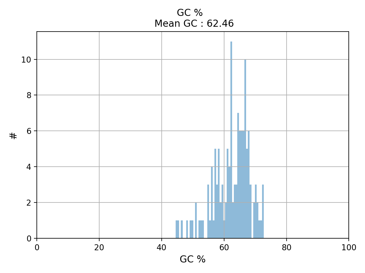
hist_GC(bins=50, alpha=0.5, hold=False, fontsize=12, grid=True, xlabel='GC %', ylabel='#', label='', title=None)#

Plot histogram GC content

Parameters:

bins (int) -- binning for the histogram
alpha (float) -- transparency of the histograms
hold (bool)
fontsize (int) -- fontsize of the x and y labels and title.
grid (bool) -- add grid or not
xlabel (str)
ylabel (str)
label (str) -- label of the histogram (for the legend)
title (str)

from sequana.pacbio import PacbioSubreads
from sequana import sequana_data
b = PacbioSubreads(sequana_data("test_pacbio_subreads.bam"))
b.hist_GC()

(Source code, png, hires.png, pdf)

hist_read_length(bins=50, alpha=0.8, hold=False, fontsize=12, grid=True, xlabel='Read Length', ylabel='#', label='', title=None, logy=False, ec='k', hist_kwargs={})#

Plot histogram Read length

Parameters:

bins (int) -- binning for the histogram
alpha (float) -- transparency of the histograms
hold (bool)
fontsize (int)
grid (bool)
xlabel (str)
ylabel (str)
label (str) -- label of the histogram (for the legend)
title (str)

from sequana.pacbio import PacbioSubreads
from sequana import sequana_data
b = PacbioSubreads(sequana_data("test_pacbio_subreads.bam"))
b.hist_read_length()

(Source code, png, hires.png, pdf)

plot_GC_read_len(hold=False, fontsize=12, bins=[200, 60], grid=True, xlabel='GC %', ylabel='#', cmap='BrBG')#

Plot GC content versus read length

Parameters:

hold (bool)
fontsize (int) -- for x and y labels and title
bins -- a integer or tuple of 2 integers to specify the binning of the x and y 2D histogram.
grid (bool)
xlabel (str)
ylabel (str)

from sequana.pacbio import PacbioSubreads
from sequana import sequana_data
b = PacbioSubreads(sequana_data("test_pacbio_subreads.bam"))
b.plot_GC_read_len(bins=[10, 10])

(Source code, png, hires.png, pdf)

reset()#

to_fasta(output_filename, threads=2)#

Export BAM reads into a Fasta file

Parameters:

output_filename -- name of the output file (use .fasta extension)
threads (int) -- number of threads to use

Note

this executes a shell command based on samtools

Warning

this takes a few minutes for 500,000 reads

to_fastq(output_filename, threads=2)#: Export BAM reads into FastQ file

class Barcoding(filename)[source]#

Read as input a file created by smrtlink that stores statistics about each barcode. This is a simple CSV file with one line per barcode<

hist_mean_polymerase_read_length(bins=10, fontsize=12)[source]#

hist_polymerase_per_barcode(bins=10, fontsize=12)[source]#

histogram of number of polymerase per barcode

Cumulative histogram gives total number of polymerase reads

hist_quality_per_barcode(bins=10, fontsize=12)[source]#

plot_and_save_all(dpi=100, directory='.')[source]#

plot_polymerase_per_barcode(fontsize=12, unbarcoded=True)[source]#: Number Of Polymerase Reads Per Barcode

plot_subreads_histogram(bins=10, fontsize=12)[source]#

class PBSim(input_bam, simul_bam)[source]#

Filter an input BAM (simulated with pbsim) so as so keep reads that fit a target distribution.

This uses a MH algorithm behind the scene.

ss = pacbio.PBSim("test10X.bam")
clf();
ss.run(bins=100, step=50)

For example, to simulate data set, use:

pbsim --data-type CLR --accuracy-min 0.85 --depth 20              --length-mean 8000 --length-sd 800 reference.fasta --model_qc model_qc_clr

The file model_qc_clr can be retrieved from the github here below.

See pfaucon/PBSIM-PacBio-Simulator for details.

We get a fastq file where simulated read sequences are randomly sampled from the reference sequence ("reference.fasta") and differences (errors) of the sampled reads are introduced.

run(bins=50, xmin=0, xmax=30000, step=1000, burn=1000, alpha=1, output_filename=None)[source]#

target_distribution(xprime)[source]#

The target distribution

Compute histogram. Get X, Y. Given xprime, interpolate to get yprime use e.g. np.interp

class PacbioMappedBAM(filename, method)[source]#

Parameters:: filename (str) -- input BAM file

boxplot_mapq_concordance()[source]#

filter_mapq(output_filename, threshold_min=0, threshold_max=255)[source]#

Select and Write reads within a given range

Parameters:

output_filename (str) -- name of output file
threshold_min (int) -- minimum length of the reads to keep
threshold_max (int) -- maximum length of the reads to keep

get_coverage(reference_length=None)[source]#

hist_GC(bins=50, alpha=0.5, hold=False, fontsize=12, grid=True, xlabel='GC %', ylabel='#', label='', title=None)#

Plot histogram GC content

Parameters:

bins (int) -- binning for the histogram
alpha (float) -- transparency of the histograms
hold (bool)
fontsize (int) -- fontsize of the x and y labels and title.
grid (bool) -- add grid or not
xlabel (str)
ylabel (str)
label (str) -- label of the histogram (for the legend)
title (str)

from sequana.pacbio import PacbioSubreads
from sequana import sequana_data
b = PacbioSubreads(sequana_data("test_pacbio_subreads.bam"))
b.hist_GC()

(Source code, png, hires.png, pdf)

hist_concordance(bins=100, fontsize=16)[source]#

formula : 1 - (in + del + mismatch / (in + del + mismatch + match) )

For BWA and BLASR, the get_cigar_stats are different !!! BWA for instance has no X stored while Pacbio forbids the use of the M (CMATCH) tag. Instead, it uses X (CDIFF) and = (CEQUAL) characters.

Subread Accuracy: The post-mapping accuracy of the basecalls. Formula: [1 - (errors/subread length)], where errors = number of deletions + insertions + substitutions.

hist_median_ccs(bins=1000, **kwargs)[source]#: Group subreads by ZMW and plot median of read length for each polymerase

hist_read_length(bins=50, alpha=0.8, hold=False, fontsize=12, grid=True, xlabel='Read Length', ylabel='#', label='', title=None, logy=False, ec='k', hist_kwargs={})#

Plot histogram Read length

Parameters:

bins (int) -- binning for the histogram
alpha (float) -- transparency of the histograms
hold (bool)
fontsize (int)
grid (bool)
xlabel (str)
ylabel (str)
label (str) -- label of the histogram (for the legend)
title (str)

from sequana.pacbio import PacbioSubreads
from sequana import sequana_data
b = PacbioSubreads(sequana_data("test_pacbio_subreads.bam"))
b.hist_read_length()

(Source code, png, hires.png, pdf)

plot_GC_read_len(hold=False, fontsize=12, bins=[200, 60], grid=True, xlabel='GC %', ylabel='#', cmap='BrBG')#

Plot GC content versus read length

Parameters:

hold (bool)
fontsize (int) -- for x and y labels and title
bins -- a integer or tuple of 2 integers to specify the binning of the x and y 2D histogram.
grid (bool)
xlabel (str)
ylabel (str)

from sequana.pacbio import PacbioSubreads
from sequana import sequana_data
b = PacbioSubreads(sequana_data("test_pacbio_subreads.bam"))
b.plot_GC_read_len(bins=[10, 10])

(Source code, png, hires.png, pdf)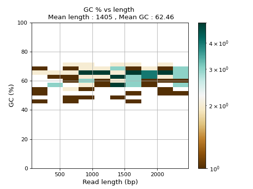

reset()#

to_fasta(output_filename, threads=2)#

Export BAM reads into a Fasta file

Parameters:

output_filename -- name of the output file (use .fasta extension)
threads (int) -- number of threads to use

Note

this executes a shell command based on samtools

Warning

this takes a few minutes for 500,000 reads

to_fastq(output_filename, threads=2)#: Export BAM reads into FastQ file

class PacbioSubreads(filename, sample=0)[source]#

BAM reader for Pacbio (reads)

You can read a file as follows:

from sequana.pacbio import Pacbiosubreads
from sequana import sequana_data
filename = sequana_data("test_pacbio_subreads.bam")
b = PacbioSubreads(filename)

A summary of the data is stored in the attribute df. It contains information such as the length of the reads, the ACGT content, the GC content.

Several plotting methods are available. For instance, hist_snr().

The BAM file used to store the Pacbio reads follows the BAM/SAM specification. Note that the sequence read are termed query, a subsequence of an entire Pacbio ZMW read ( a subread), which is basecalls from a single pass of the insert DNA molecule.

In general, only a subsequence of the query will align to the reference genome, and that subsequence is referred to as the aligned query.

When introspecting the aligned BAM file, the extent of the query in ZMW read is denoted as [qStart, qEnd) and the extent of the aligned subinterval as [aStart, aEnd). The following graphic illustrates these intervals:

      qStart                         qEnd
0         |  aStart                aEnd  |
[--...----*--*---------------------*-----*-----...------)  < "ZMW read" coord. system
          ~~~----------------------~~~~~~                  <  query; "-" =aligning subseq.
[--...-------*---------...---------*-----------...------)  < "ref." / "target" coord. system
0            tStart                tEnd

In the BAM files, the qStart, qEnd are contained in the qs and qe tags, (and reflected in the QNAME); the bounds of the aligned query in the ZMW read can be determined by adjusting qs and qe by the number of soft-clipped bases at the ends of the alignment (as found in the CIGAR).

See also the comments in the code for other tags.

Reference:: http://pacbiofileformats.readthedocs.io/en/3.0/BAM.html

Constructor

Parameters:

filename (str) -- filename of the input pacbio BAM file. The content of the BAM file is not the ouput of a mapper. Instead, it is the output of a Pacbio (Sequel) sequencing (e.g., subreads).
sample (int) -- for sample, you can set the number of subreads to read (0 means read all subreads)

boxplot_read_length_vs_passes(nmax=20, ax=None, whis=1.5, widths=0.6)[source]#

property df#

filter_length(output_filename, threshold_min=0, threshold_max=inf)[source]#

Select and Write reads within a given range

Parameters:

output_filename (str) -- name of output file
threshold_min (int) -- minimum length of the reads to keep
threshold_max (int) -- maximum length of the reads to keep

get_mean_nb_passes(min_length=50, max_length=1500000)[source]#

get_number_of_ccs(min_length=50, max_length=1500000)[source]#

Return number of CCS reads within a given range

This is useful for subreads where no CCS are computed but ZMW can give an estimation of number of unique possible CCS

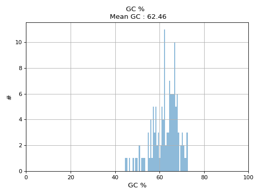
hist_GC(bins=50, alpha=0.5, hold=False, fontsize=12, grid=True, xlabel='GC %', ylabel='#', label='', title=None)#

Plot histogram GC content

Parameters:

bins (int) -- binning for the histogram
alpha (float) -- transparency of the histograms
hold (bool)
fontsize (int) -- fontsize of the x and y labels and title.
grid (bool) -- add grid or not
xlabel (str)
ylabel (str)
label (str) -- label of the histogram (for the legend)
title (str)

from sequana.pacbio import PacbioSubreads
from sequana import sequana_data
b = PacbioSubreads(sequana_data("test_pacbio_subreads.bam"))
b.hist_GC()

(Source code, png, hires.png, pdf)

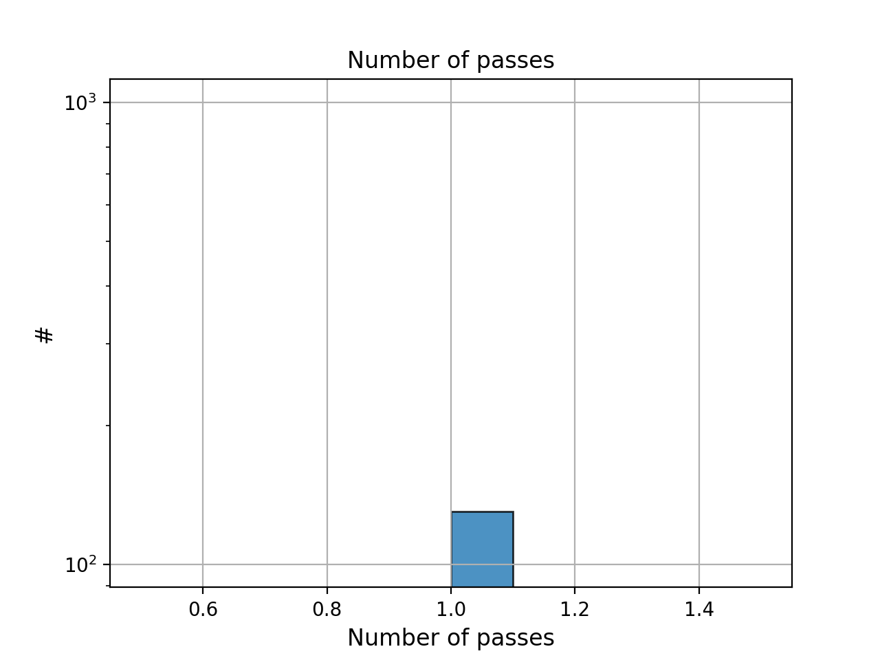
hist_nb_passes(bins=None, alpha=0.8, hold=False, fontsize=12, grid=True, xlabel='Number of passes', logy=True, ec='k', ylabel='#', label='', title='Number of passes')[source]#

Plot histogram of number of passes

Parameters:

alpha (float) -- transparency of the histograms
hold (bool)
fontsize (int)
grid (bool)
xlabel (str)
ylabel (str)
logy (bool) -- use log scale on the y axis (default to True)
label (str) -- label of the histogram (for the legend)
title (str)

from sequana.pacbio import PacbioSubreads
from sequana import sequana_data
b = PacbioSubreads(sequana_data("test_pacbio_subreads.bam"))
b.hist_nb_passes()

(Source code, png, hires.png, pdf)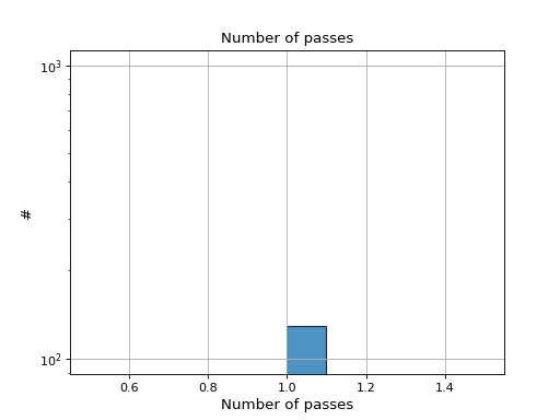

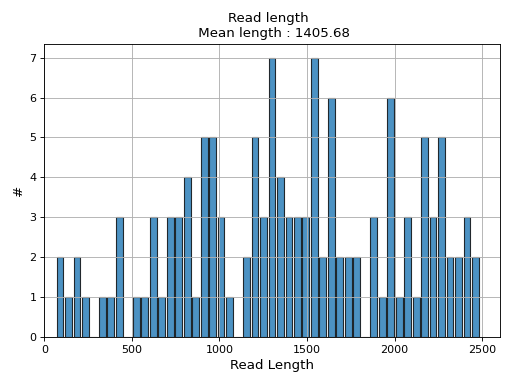
hist_read_length(bins=50, alpha=0.8, hold=False, fontsize=12, grid=True, xlabel='Read Length', ylabel='#', label='', title=None, logy=False, ec='k', hist_kwargs={})#

Plot histogram Read length

Parameters:

bins (int) -- binning for the histogram
alpha (float) -- transparency of the histograms
hold (bool)
fontsize (int)
grid (bool)
xlabel (str)
ylabel (str)
label (str) -- label of the histogram (for the legend)
title (str)

from sequana.pacbio import PacbioSubreads
from sequana import sequana_data
b = PacbioSubreads(sequana_data("test_pacbio_subreads.bam"))
b.hist_read_length()

(Source code, png, hires.png, pdf)

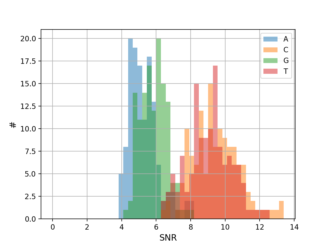
hist_snr(bins=50, alpha=0.5, hold=False, fontsize=12, grid=True, xlabel='SNR', ylabel='#', title='', clip_upper_SNR=30)[source]#

Plot histogram of the ACGT SNRs for all reads

Parameters:

bins (int) -- binning for the histogram. Note that the range starts at 0 and ends at clip_upper_SNR
alpha (float) -- transparency of the histograms
hold (bool)
fontsize (int)
grid (bool)
xlabel (str)
ylabel (str)
title (str)

from sequana.pacbio import PacbioSubreads
from sequana import sequana_data
b = PacbioSubreads(sequana_data("test_pacbio_subreads.bam"))
b.hist_snr()

(Source code, png, hires.png, pdf)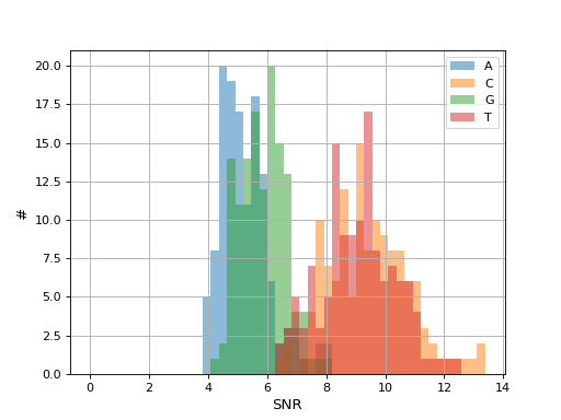

plot_GC_read_len(hold=False, fontsize=12, bins=[200, 60], grid=True, xlabel='GC %', ylabel='#', cmap='BrBG')#

Plot GC content versus read length

Parameters:

hold (bool)
fontsize (int) -- for x and y labels and title
bins -- a integer or tuple of 2 integers to specify the binning of the x and y 2D histogram.
grid (bool)
xlabel (str)
ylabel (str)

from sequana.pacbio import PacbioSubreads
from sequana import sequana_data
b = PacbioSubreads(sequana_data("test_pacbio_subreads.bam"))
b.plot_GC_read_len(bins=[10, 10])

(Source code, png, hires.png, pdf)

random_selection(output_filename, nreads=None, expected_coverage=None, reference_length=None, read_lengths=None)[source]#

Select random reads

Parameters:

nreads -- number of reads to select randomly. Must be less than number of available reads in the orignal file.
expected_coverage
reference_length

if expected_coverage and reference_length provided, nreads is replaced automatically.

Note

to speed up computation (if you need to call random_selection many times), you can provide the mean read length manually

reset()#

save_summary(filename)[source]#

property stats#: return basic stats about the read length

stride(output_filename, stride=10, shift=0, random=False)[source]#

Write a subset of reads to BAM output

Parameters:

output_filename (str) -- name of output file
stride (int) -- optionnal, number of reads to read to output one read
shift (int) -- number of reads to ignore at the begining of input file
random (bool) -- if True, at each step the read to output is randomly selected

summary()[source]#

to_fasta(output_filename, threads=2)#

Export BAM reads into a Fasta file

Parameters:

output_filename -- name of the output file (use .fasta extension)
threads (int) -- number of threads to use

Note

this executes a shell command based on samtools

Warning

this takes a few minutes for 500,000 reads

to_fastq(output_filename, threads=2)#: Export BAM reads into FastQ file

Pacbio amplicon related tools

class Consensus(bases, freebayes=None)[source]#

get_bases()[source]#

get_population(threshold=0.1, Npop=2)[source]#

identify_deletions()[source]#

run()[source]#

save_consensus(output, identifier)[source]#

class LAA(where='bc*')[source]#

Reads a set of file called amplicon_summary.csv generated by the LAA pipeline from smrtlink pacbio tool.

The file have this format:

BarcodeName,FastaName,CoarseCluster,Phase,TotalCoverage,SequenceLength,PredictedAccuracy,ConsensusConverged,NoiseSequence,IsDuplicate,DuplicateOf,IsChimera,ChimeraScore,ParentSequenceA,ParentSequenceB,CrossoverPosition
24--24,Barcode24--24_Cluster0_Phase0_NumReads497,0,0,497,2958,1,1,0,0,N/A,0,-1,N/A,N/A,-1
24--24,Barcode24--24_Cluster1_Phase0_NumReads496,1,0,496,3137,1,1,0,0,N/A,0,-1,N/A,N/A,-1

See plot_max_length_amplicon_per_barcode() for some details about sample names.

hist_amplicon(fontsize=12)[source]#

plot_max_length_amplicon_per_barcode(sample_names=None)[source]#

Plot max length of the amplicons per barcode

Parameters:: sample_names -- names of the barcode. If not provided use number from 1 to N. See below.

One difficulty here is to associate a file with a barcode name. The files created by LAA have the same basename and the content of the file cannot be parsed to obtain the barcode (indeed some may be empty). So, we need to provide a list of sample names in plot_max_length_amplicon_per_barcode() associated to the files. Otherwise a simple range of names from 1 to N is used.

class LAA_Assembly(filename)[source]#

Input is a SAM/BAM from the mapping of amplicon onto a known reference. Based on the position, we can construct the new reference.

build_reference()[source]#

save_fasta(filename, sequence=None)[source]#

class IsoSeqBAM(filename)[source]#

Reads raw IsoSeq BAM file (subreads)

Creates some plots and stats

hist_passes(bins=100)[source]#

hist_read_length(bins=100)[source]#

property lengths#

property passes#

stats()[source]#

class IsoSeqQC(directory='.', prefix='')[source]#

Use get_isoseq_files on smrtlink to get the proper files

iso = IsoSeqQC() iso.hist_read_length_consensus_isoform() # histo CCS iso.stats() # "CCS" key is equivalent to summary metrics in CCS report

todo: get CCS passes histogram . Where to get the info of passes ?

get_file(tag, noprefix=False)[source]#

hist_average_quality(fontsize=16, bins=None)[source]#: bins is from 0 to 94

hist_read_length_consensus_isoform(mode='all', bins=80, rwidth=0.8, align='left', fontsize=16, edgecolor='k', **kwargs)[source]#: mode can be all, lq, hq

stats()[source]#

to_summary(filename='sequana_summary_isoseq.json', data=None)[source]#

Save statistics into a JSON file

Parameters:

filename
data -- dictionary to save. If not provided, use stats()

LAA tools (pacbio)

class Consensus(bases, freebayes=None)[source]#

get_bases(skip_rows=3)[source]#

get_population(threshold=0.1, Npop=2)[source]#

identify_deletions()[source]#

run()[source]#

save_consensus(output, identifier)[source]#

split_according_to_reference_name(prefix='consensus')[source]#

class LAA(where='bc*')[source]#

Reads a set of file called amplicon_summary.csv generated by the LAA pipeline from smrtlink pacbio tool.

The file have this format:

BarcodeName,FastaName,CoarseCluster,Phase,TotalCoverage,SequenceLength,PredictedAccuracy,ConsensusConverged,NoiseSequence,IsDuplicate,DuplicateOf,IsChimera,ChimeraScore,ParentSequenceA,ParentSequenceB,CrossoverPosition
24--24,Barcode24--24_Cluster0_Phase0_NumReads497,0,0,497,2958,1,1,0,0,N/A,0,-1,N/A,N/A,-1
24--24,Barcode24--24_Cluster1_Phase0_NumReads496,1,0,496,3137,1,1,0,0,N/A,0,-1,N/A,N/A,-1

See plot_max_length_amplicon_per_barcode() for some details about sample names.

hist_amplicon(fontsize=12)[source]#

plot_max_length_amplicon_per_barcode(sample_names=None)[source]#

Plot max length of the amplicons per barcode

Parameters:: sample_names -- names of the barcode. If not provided use number from 1 to N. See below.

class LAA_Assembly(filename)[source]#

Input is a SAM/BAM from the mapping of amplicon onto a known reference. Based on the position, we can construct the new reference.

build_reference()[source]#

save_fasta(filename, sequence=None)[source]#

RNA-seq / counting #

class RNADesign(filename, sep='\\s*,\\s*', condition_col='condition', reference=None)[source]#

Simple RNA design handler

checker()[source]#

property comparisons#

property conditions#

keep_conditions(conditions)[source]#

validate()[source]#

class RNADiffAnalysis(counts_file, design_file, condition, keep_all_conditions=False, reference=None, comparisons=None, batch=None, fit_type='parametric', beta_prior=False, independent_filtering=True, cooks_cutoff=None, gff=None, fc_attribute=None, fc_feature=None, annot_cols=None, threads=4, outdir='rnadiff', sep_counts=',', sep_design='\\s*,\\s*', minimum_mean_reads_per_gene=0, minimum_mean_reads_per_condition_per_gene=0, model=None)[source]#

A tool to prepare and run a RNA-seq differential analysis with DESeq2

Parameters:

counts_file -- Path to tsv file out of FeatureCount with all samples together.
design_file -- Path to tsv file with the definition of the groups for each sample.
condition -- The name of the column from groups_tsv to use as condition. For more advanced design, a R function of the type 'condition*inter' (without the '~') could be specified (not tested yet). Each name in this function should refer to column names in groups_tsv.
comparisons -- A list of tuples indicating comparisons to be made e.g A vs B would be [("A", "B")]
batch -- None for no batch effect or name of a column in groups_tsv to add a batch effect.
keep_all_conditions -- if user set comparisons, it means will only want to include some comparisons and therefore their conditions. Yet, sometimes, you may still want to keep all conditions in the diffential analysis. If some set this flag to True.
fit_type -- Default "parametric".
beta_prior -- Default False.
independent_filtering -- To let DESeq2 perform the independentFiltering or not.
cooks_cutoff -- To let DESeq2 decide for the CooksCutoff or specifying a value.
gff -- Path to the corresponding gff3 to add annotations.
fc_attribute -- GFF attribute used in FeatureCounts.
fc_feature -- GFF feaure used in FeatureCounts.
annot_cols -- GFF attributes to use for results annotations
threads -- Number of threads to use
outdir -- Path to output directory.
sep_counts -- The separator used in the input count file.
sep_design -- The separator used in the input design file.

This class reads a sequana.featurecounts.

r = rnadiff.RNADiffAnalysis("counts.csv", "design.csv",
        condition="condition", comparisons=[(("A", "B"), ('A', "C")],

For developers: the rnadiff_template.R script behind the scene expects those attributes to be found in the RNADiffAnalysis class: counts_filename, design_filename, fit_type, fonction, comparison_str, independent_filtering, cooks_cutoff, code_dir, outdir, counts_dir, beta_prior, threads

check_and_save_input_tables(sep_counts)[source]#

check_comparisons()[source]#

run()[source]#

Create outdir and a DESeq2 script from template for analysis. Then execute this script.

Returns:: a RNADiffResults instance

template = <Template 'rnadiff_light_template.R'>#

class RNADiffResults(rnadiff_folder, gff=None, fc_attribute=None, fc_feature=None, pattern='*vs*_degs_DESeq2.csv', alpha=0.05, log2_fc=0, palette=None, condition='condition', annot_cols=None, **kwargs)[source]#

The output of a RNADiff analysis

Rnadiff_folder:: a valid rnadiff folder created by RNADiffAnalysis

RNADiffResults("rnadiff/")

property alpha#

get_gene_lists(annot_col='index', Nmax=None, dropna=False)[source]#

heatmap(comp, log2_fc=1, padj=0.05)[source]#

heatmap_vst_centered_data(comp, log2_fc=1, padj=0.05, xlabel_size=8, ylabel_size=12, figsize=(10, 15), annotation_column=None)[source]#

import_tables()[source]#

property log2_fc#

plot_boxplot_normeddata(fliersize=2, linewidth=2, rotation=0, fontsize=None, xticks_fontsize=None, **kwargs)[source]#

plot_boxplot_rawdata(fliersize=2, linewidth=2, rotation=0, fontsize=None, xticks_fontsize=None, **kwargs)[source]#

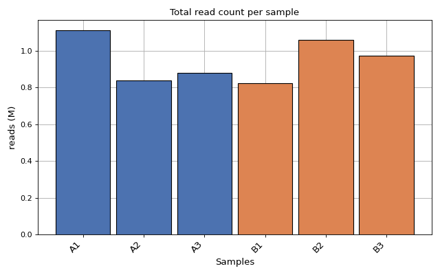
plot_count_per_sample(fontsize=None, rotation=45, xticks_fontsize=None)[source]#

Number of mapped and annotated reads (i.e. counts) per sample. Each color for each replicate

from sequana.rnadiff import RNADiffResults
from sequana import sequana_data

r = RNADiffResults(sequana_data("rnadiff/", "doc"))
r.plot_count_per_sample()

(Source code, png, hires.png, pdf)

plot_dendogram(max_features=5000, transform_method='log', method='ward', metric='euclidean', count_mode='norm')[source]#

plot_density()[source]#

plot_dispersion()[source]#

plot_feature_most_present(fontsize=None, xticks_fontsize=None)[source]#

Bar plot of the most expressed feature per sample.

For each sample, identifies the feature with the highest raw count and displays the percentage of total counts attributed to that feature.

plot_isomap(n_components=2, colors=None)[source]#: IN DEV, not functional

plot_mds(n_components=2, colors=None, clf=True)[source]#: IN DEV, not functional

plot_most_expressed_features(N=20)[source]#

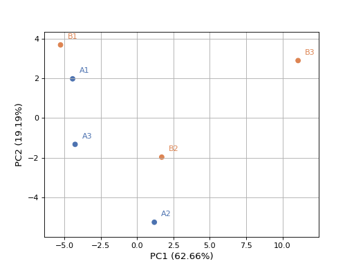
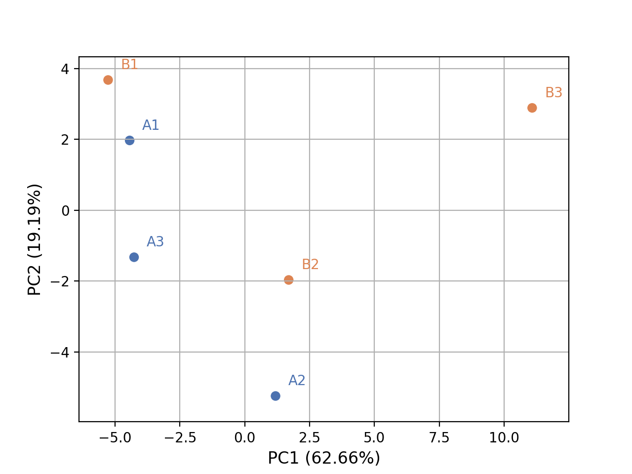
plot_pca(n_components=2, colors=None, plotly=False, max_features=500, genes_to_remove=[], fontsize=10, adjust=True, transform_method='none', count_mode='vst')[source]#

from sequana.rnadiff import RNADiffResults
from sequana import sequana_data

r = RNADiffResults(sequana_data("rnadiff/", "doc"))

colors = {
    'surexp1': 'r',
    'surexp2':'r',
    'surexp3':'r',
    'surexp1': 'b',
    'surexp2':'b',
    'surexp3':'b'}
r.plot_pca(colors=colors)

(Source code, png, hires.png, pdf)

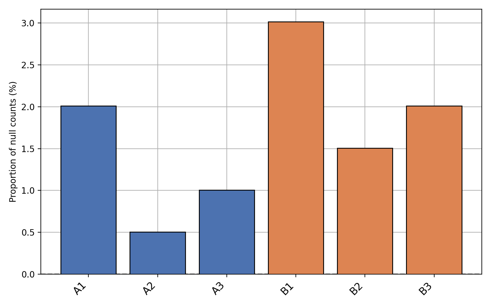
plot_percentage_null_read_counts(fontsize=None, xticks_fontsize=None)[source]#

Bars represent the percentage of null counts in each samples. The dashed horizontal line represents the percentage of feature counts being equal to zero across all samples

from sequana.rnadiff import RNADiffResults
from sequana import sequana_data

r = RNADiffResults(sequana_data("rnadiff/", "doc"))
r.plot_percentage_null_read_counts()

(Source code, png, hires.png, pdf)

plot_upset(force=False, max_subsets=20)[source]#

Plot the upset plot (alternative to venn diagram).

with many comparisons, plots may be quite large. We can reduce the width by ignoring the small subsets. We fix the max number of subsets to 20 for now.

read_annot(gff)[source]#

Get a properly formatted dataframe from the gff.

Parameters:: gff -- a input GFF filename or an existing instance of GFF3

read_csv(filename)[source]#

report()[source]#

summary()[source]#

to_csv(filename)[source]#

class RNADiffTable(path, alpha=0.05, log2_fc=0, sep=',', condition='condition', shrinkage=True)[source]#

A representation of the results of a single rnadiff comparison

Expect to find output of RNADiffAnalysis file named after condt1_vs_cond2_degs_DESeq2.csv

from sequana.rnadiff import RNADiffTable
RNADiffTable("A_vs_B_degs_DESeq2.csv")

property alpha#

filter()[source]#: filter a DESeq2 result with FDR and logFC thresholds

property log2_fc#

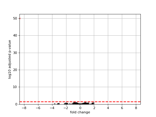
plot_padj_hist(bins=60, fontsize=16)[source]#

plot_pvalue_hist(bins=60, fontsize=16, rotation=0)[source]#

plot_volcano(padj=0.05, add_broken_axes=False, markersize=4, limit_broken_line=[20, 40], plotly=False, annotations=None, hover_name=None)[source]#

from sequana.rnadiff import RNADiffResults
from sequana import sequana_data

r = RNADiffResults(sequana_data("rnadiff/", "doc"))
r.comparisons["A_vs_B"].plot_volcano()

(Source code, png, hires.png, pdf)

set_gene_lists()[source]#

summary()[source]#

class RNADiffCompare(*args, design=None)[source]#

An object representation of results coming from a RNADiff analysis.

from sequana.compare import RNADiffCompare
c = RNADiffCompare("data.csv", "data2.csv")

# change the l2fc to update venn plots
c.plot_venn_up()
c.r1.log2_fc = 1
c.r2.log2_fc = 1
c.plot_venn_up()

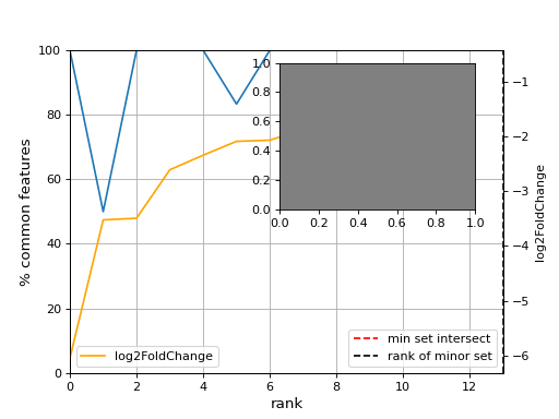
plot_common_major_counts(mode, labels=None, switch_up_down_cond2=False, add_venn=True, xmax=None, title='', fontsize=12, sortby='log2FoldChange')[source]#

Parameters:: mode -- down, up or all

from sequana import sequana_data
from sequana.compare import RNADiffCompare

c = RNADiffCompare(
    sequana_data("rnadiff_salmon.csv", "doc/rnadiff_compare"),
    sequana_data("rnadiff_bowtie.csv", "doc/rnadiff_compare")
)
c.plot_common_major_counts("down")

(Source code)

_images/references_pipelines-39_00.png — (`png`, `hires.png`, `pdf`)#

_images/references_pipelines-39_01.png — (`png`, `hires.png`, `pdf`)#

plot_corrplot_counts_normed(samples=None, log2=True, lower='pie', upper='text')[source]#

plot_corrplot_counts_raw(samples=None, log2=True, lower='pie', upper='text')[source]#

plot_foldchange()[source]#

plot_geneset(indices, showlines=True, showdots=True, colors={'bodies': 'blue', 'cbars': 'k', 'cmaxes': 'k', 'cmins': 'k', 'dot': 'blue'})[source]#

indices is a list that represents a gene sets

cmins, cmaxes, cbars are the colors of the bars inside the body of the violin plots

(Source code, png, hires.png, pdf)

plot_jaccard_distance(mode, padjs=[0.0001, 0.001, 0.01, 0.05, 0.1], Nfc=50, smooth=False, window=5)[source]#

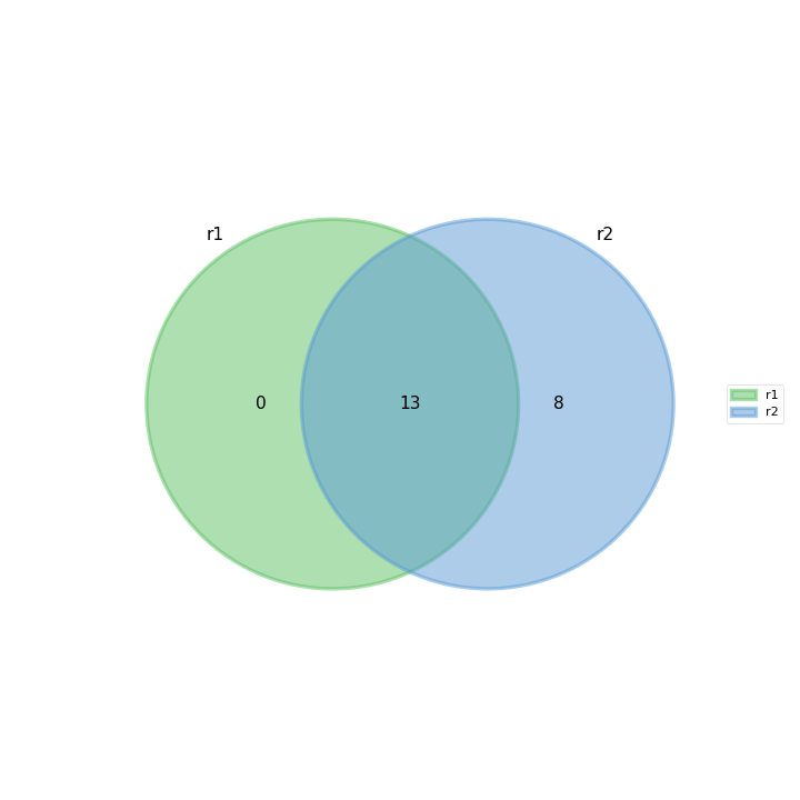
plot_venn_all(labels=None, ax=None, title='all expressed genes', mode='all')[source]#

plot_venn_down(labels=None, ax=None, title='Down expressed genes', mode='all', l2fc=0)[source]#

plot_venn_up(labels=None, ax=None, title='Up expressed genes', mode='all', l2fc=0)[source]#

Venn diagram of cond1 from RNADiff result1 vs cond2 in RNADiff result 2

from sequana import sequana_data
from sequana.compare import RNADiffCompare

c = RNADiffCompare(
    sequana_data("rnadiff_salmon.csv", "doc/rnadiff_compare"),
    sequana_data("rnadiff_bowtie.csv", "doc/rnadiff_compare")
)
c.plot_venn_up()

(Source code, png, hires.png, pdf)

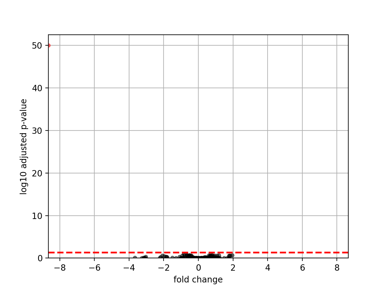
plot_volcano(labels=None)[source]#

Volcano plot of log2 fold change versus log10 of adjusted p-value

from sequana import sequana_data
from sequana.compare import RNADiffCompare

c = RNADiffCompare(
    sequana_data("rnadiff_salmon.csv", "doc/rnadiff_compare"),
    sequana_data("rnadiff_bowtie.csv", "doc/rnadiff_compare")
)
c.plot_volcano()

(Source code, png, hires.png, pdf)

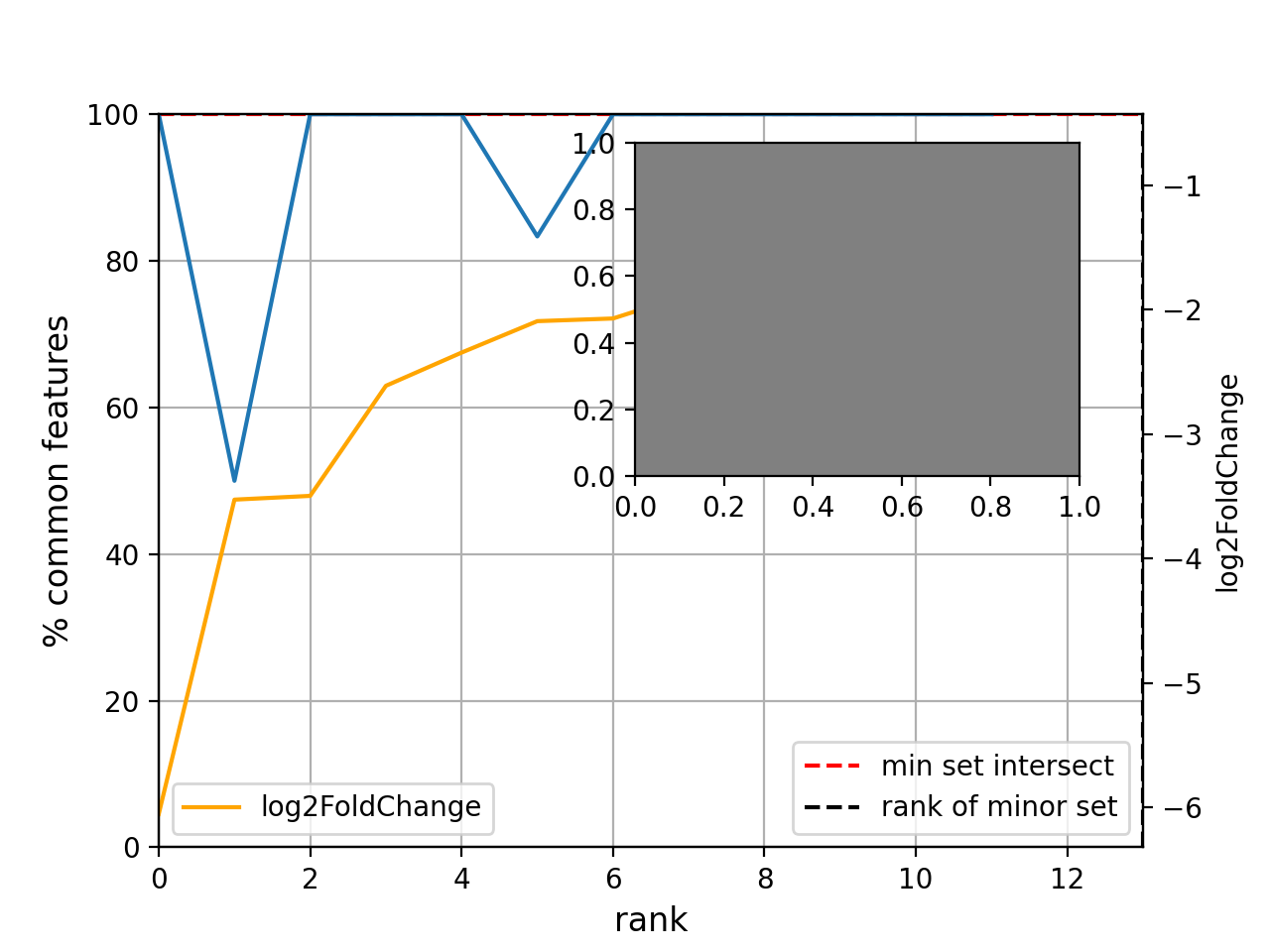
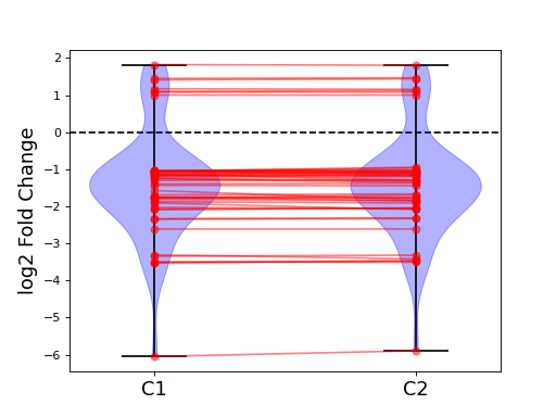
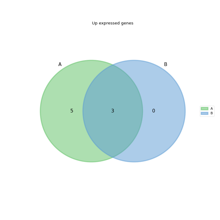
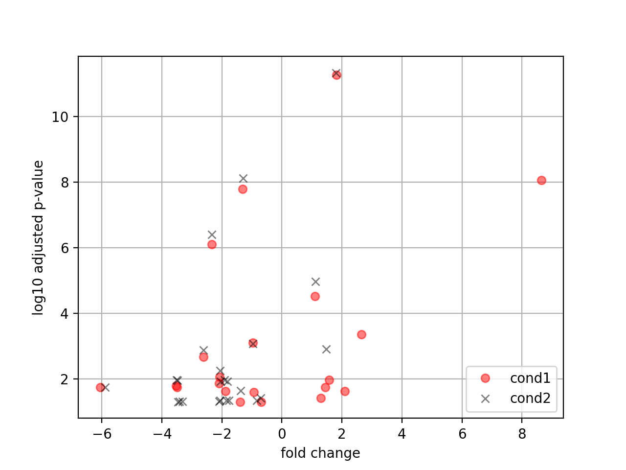
plot_volcano_differences(mode='all')[source]#

feature counts related tools

class FeatureCount(filename, clean_sample_names=True, extra_name_rm=['_Aligned'], drop_loc=True, guess_design=False)[source]#

Read a featureCounts output file.

The input file is expected to be generated with featurecounts tool. It should be a TSV file such as the following one with the header provided herebelow. Of course input BAM files can be named after your samples:

Geneid    Chr    Start    End    Strand    Length    WT1    WT2 WT3 KO1 KO2 KO3
gene1    NC_010602.1    141    1466    +    1326    11    20    15    13    17    17
gene2    NC_010602.1    1713    2831    +    1119    35    54    58    34    53    46
gene3    NC_010602.1    2831    3934    +    1104    9    16    16    4    18    18

from sequana import FeatureCount
fc = FeatureCount("all_features.out", extra_name_rm=["_S\d+"]
fc.rnadiff_df.to_csv("fc.csv")

Constructor

Get the featureCounts output as a pandas DataFrame

Parameters:

clean_sample_names (bool) -- if simplifying the sample names in featureCount output columns
extra_name_rm (list) -- extra list of regex to remove from samples_names (ignored if clean_sample_name is False)
drop_loc (bool) -- if dropping the extra location columns (ie getting only the count matrix)

property df#

class FeatureCountMerger(pattern='*feature.out', fof=[], skiprows=1)[source]#

Merge several feature counts files

to_tsv(output_filename='all_features.out')[source]#

class MultiFeatureCount(rnaseq_folder='.', tolerance=0.1)[source]#

Read set of feature counts using different options of strandness

from sequana import sequana_data
from sequana.featurecounts import *
directory = sequana_data("/rnaseq_0")
ff = MultiFeatureCount(directory, 0.15)
ff._get_most_probable_strand_consensus()
ff.plot_strandness()

(Source code, png, hires.png, pdf)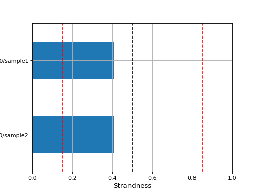

See also

get_most_probable_strand() for more information about the tolerance parameter and meaning of strandness.

The expected data structure is

rnaseq_folder
├── sample1
│   ├── feature_counts_0
│   │   └── sample_feature.out
│   ├── feature_counts_1
│   │   └── sample_feature.out
│   ├── feature_counts_2
│   │   └── sample_feature.out
└── sample2
    ├── feature_counts_0
    │   └── sample_feature.out
    ├── feature_counts_1
    │   └── sample_feature.out
    ├── feature_counts_2
    │   └── sample_feature.out

The new expected data structure is

new_rnaseq_output/
├── sample1
│   └── feature_counts
│       ├── 0
│       │   └── sample_feature.out
│       ├── 1
│       │   └── sample_feature.out
│       └── 2
│           └── sample_feature.out
└── sample2
    └── feature_counts
        ├── 0
        │   └── sample_feature.out
        ├── 1
        │   └── sample_feature.out
        └── 2
            └── sample_feature.out

Parameters:

rnaseq_folder (str)
tolerance (int) -- the tolerance between 0 and 0.25

plot_strandness(fontsize=12, output_filename='strand_summary.png', savefig=False)[source]#

get_most_probable_strand(filenames, tolerance, sample_name)[source]#

Return most propable strand given 3 feature count files (strand of 0,1, and 2)

Return the total counts by strand from featureCount matrix folder, strandness and probable strand for a single sample (using a tolerance threshold for strandness). This assumes a single sample by featureCounts file.

Parameters:

filenames -- a list of 3 feature counts files for a given sample corresponding to the strand 0,1,2
tolerance -- a value below 0.5
sample -- the name of the sample corresponding to the list in filenames

Possible values returned are:

0: unstranded
1: stranded
2: eversely stranded

We compute the number of counts in case 1 and 2 and compute the ratio strand as $RS = stranded / (stranded + reversely stranded )$ . Then we decide on the possible strandness with the following criteria:

if RS < tolerance, reversely stranded
if RS in 0.5+-tolerance: unstranded.
if RS > 1-tolerance, stranded
otherwise, we cannot decided.

get_most_probable_strand_consensus(rnaseq_folder, tolerance, sample_pattern='*/feature_counts_[012]', file_pattern='feature_counts_[012]/*_feature.out')[source]#

From a sequana RNA-seq run folder get the most probable strand, based on the frequecies of counts assigned with '0', '1' or '2' type strandness (featureCounts nomenclature) across all samples.

Parameters:

rnaseq_folder -- the main directory
tolerance -- a value in the range 0-0.5. typically 0.1 or 0.15
pattern -- the samples directory pattern
pattern_file -- the feature counts pattern

If guess is not possible given the tolerance, fills with None

Consider this tree structure:

rnaseq_folder
├── sample1
│   └── feature_counts
│       ├── 0
│       │   └── sample_feature.out
│       ├── 1
│       │   └── sample_feature.out
│       └── 2
│           └── sample_feature.out
└── sample2
    └── feature_counts
        ├── 0
        │   └── sample_feature.out
        ├── 1
        │   └── sample_feature.out
        └── 2
            └── sample_feature.out

Then, the following command should all files and report the most probable strand (0,1,2) given the sample1 and sample2:

get_most_probable_strand_consensus("rnaseq_folder", 0.15)

This tree structure is understood automatically. If you have a different one, you can set the pattern (for samples) and pattern_files parameters.

class Salmon(filename, gff_input, attribute='transcript_id')[source]#

Factory to read counts from salmon and create feature counts usable for deseq2

get_feature_counts(feature=None, attribute=None)[source]#

get_feature_counts_eukaryotes(feature=None, attribute=None)[source]#

get_feature_counts_prokaryotes(feature=None, attribute=None)[source]#

save_feature_counts(filename, feature='gene', attribute='ID')[source]#

Variants / annotation #

Tools to launch snpEff.

class SnpEff(annotation, log=None, snpeff_datadir='data', fastafile=None, build_options='')[source]#

SnpEff is a tool dedicated to annotate detected variants in a VCF file. This wrapper eases the annotation with a genbank file. It create automatically the custom database. Then, run snpEff with a subprocess. Caution, the locus name (or chromosome name) in genbank file and the sequence name in VCF file must be the same. Otherwise, snpEff is not able to bind informations.

Example:

snpeff = SnpEff('file.gbk')
snpeff.launch_snpeff('variants.vcf', 'variant.ann.vcf')

If your input is in GFF format, you must also provide the fasta reference file.

Will save relevant snpeff data into ./data directory (or snpeff_datadir).

Constructor

Parameters:

annotation -- annotation reference.
file_format -- format of your file. ('only genbank actually')
log -- log file
snpeff_datadir -- default to data.
fastafile -- if a GFF is used, you must provide the FASTA input file as well

add_locus_in_fasta(fasta, output_file)[source]#

Add locus of annotation file in description line of fasta file. If fasta file and genbank file do not have the same names.

Parameters:

fasta (str) -- input fasta file where you want to add locus.
output_file (str) -- output file.

FIXME: fasta is already known if provided in the init

launch_snpeff(vcf_filename, output, html_output=None, options='')[source]#

Launch snpEff with the custom genbank file.

Parameters:

vcf_filename (str) -- input VCF filename.
output (str) -- output VCF filename.
html_output (str) -- filename of the HTML creates by snpEff.
options (str) -- any options recognised by snpEff.

download_fasta_and_genbank(identifier, tag, genbank=True, fasta=True, outdir='.')[source]#

Parameters:

identifier -- valid identifier to retrieve from NCBI (genbank) and ENA (fasta)
tag -- name of the filename for the genbank and fasta files.

class CNVnator(filename)[source]#

Reader of the CNVnator output file.

hist_event_size(bins=20)[source]#

plot(chr_name, x1=None, x2=None, Y=20)[source]#

class SomyScore("file.bam") ss.run() # filters ss.remove_outliers() ss.remove_flanking_regions() ss.boxplot()[source]#

# store df for later df = ss.df.copy()

ss2.run(mapq=35) # filters ss.remove_outliers() ss.remove_flanking_regions() ss.boxplot()

ss.df = pd.merge(ss.df, df) ss.boxplot()

boxplot(legend=False, hlines=[1, 1.5, 2, 2.5], normalise=True, k=None, muhat=None, hybrid=False, method='em', palette=None)[source]#

Parameters:: legend (bool) -- set to 'auto' to add a legend

compute_coverage(use_median=True, fast=True, mapq=0, flag=1796, chromosomes=None, tag='default', threads=4, exclude_chromosomes=[])[source]#

property df#

plot_filter_stats(filename='sequana_filter_stats.png')[source]#

remove_flanks(remove_flanking_regions_kb=10)[source]#

remove_low_depth(threshold=10)[source]#

remove_outliers(percentile=0.05)[source]#

ChIP-seq / peak calling #

class MACS3Reader(filename)[source]#

This class reads output of macs3 tool

from sequana import MACS3Reader
mr = MACS3Reader(data)
mr.df
mr.plot_volcano()

If input file ends in .xls, we assume this is a NAME_peaks.xls file. It is therefore a tabulated file where columns are:

chromosome name
start position of peak
end position of peak
length of peak region
absolute peak summit position
pileup height at peak summit
-log10(pvalue) for the peak summit (e.g. pvalue =1e-10, then this value should be 10)
fold enrichment for this peak summit against random Poisson distribution with local lambda,
-log10(qvalue) at peak summit

Note that coordinates in XLS is 1-based which is different from BED format that follows. When --broad is enabled for broad peak calling, the pileup, p-value, q-value, and fold change in the XLS file will be the mean value across the entire peak region, since peak summit won't be called in broad peak calling mode.

NAME_peaks.narrowPeak is BED6+4 format file which contains the peak locations together with peak summit, p-value, and q-value.

The fifth column is the score calculate as int(-10*log10_pvalue) or int(-10*log10_pvalue) where log10-pvalue/log10-qvalue is the 8th or 9th column depending on whether -p (pvalue) or -q (qvalue) is used as score cutoff. The 7th columns stores the fold-change at peak summit. The 8th is -log10pvalue at peak summit and the 9th is -log10qvalue at peak summit. The 10th is the relative summit position to peak start equivalent to absolute peak summit position in the xls file.

NAME_peaks.broadPeak is in BED6+3 format which is similar to narrowPeak file, except for missing the 10th column for annotating peak summits. This file and the gappedPeak file will only be available when --broad is enabled. Since in the broad peak calling mode, the peak summit won't be called, the values in the 5th, and 7-9th columns are the mean value across all positions in the peak region. Refer to narrowPeak if you want to fix the value issue in the 5th column

Reference: macs3-project/MACS

plot_volcano(plotly=False, marker_color='b', title='')[source]#: Plots -log10 p-value versus fold change of all peaks

class PeakConsensus(f1, f2)[source]#

merge(overlap=0.2)[source]#

plot_venn(title='', labels=[])[source]#

to_bed(filename)[source]#

to_saf(filename)[source]#: For now, all strand are categorised as strand + . strand not used in the pipeline for now.

class Homer(filename)[source]#

pie_annotation(wedgeprops={'ec': 'k'}, **kwargs)[source]#

class IDR(filename, threshold=0.05)[source]#

Reader for the output generated by idr package

Can read the narrow or broad output transparently.

Note that signalValue = rep1_signal + rep2_signal

The score columns contains the scaled IDR value, min(int(log2(-125IDR), 1000). This means that peaks with an IDR of 0 have a score of 1000. A peak with an IDR of 0.05 has a score of int(-125log2(0.05)) = 540. Finally, a peaks with an IDR of 1.0 have a score of 0. Examples:

IDR, score
0039, 1000
01, 830
05, 540
1, 415
5, 125

This allows to differentiate those that crosses an IDR or 0.05. The final IDR is stored in global_idr

IDR2score(IDR)[source]#

property N_significant_peaks#

property mode#

plot_idr_vs_peaks(filename=None, savefig=False)[source]#

plot_rank_vs_idr_score(filename=None, savefig=False)[source]#

plot_ranks(filename=None, savefig=False)[source]#

plot_scores(filename=None, savefig=False)[source]#

score2IDR(score)[source]#

class FRiP(filename)[source]#

Reader for output of FRiP computation in chipseq pipeline

FRiP is the fraction of reads found in Peaks.

expected format:

bamfile,count,in_peaks,FRiP
1_S1_L001.sorted.bam,3548090,53673,0.01512729383978422
2_S2_L001.sorted.bam,3868608,58292,0.01506795209026089
3_S3_L001.sorted.bam,4092990,50219,0.01226951446253228

plot()[source]#: scatter plot of FRiP versus Reads in peaks

class Phantom(bamfile=None, binning=5, start=-500, stop=1500)[source]#

Read alignment files and generated phantom peaks.

This class reads align files generated from bam files using this set of commands:

samtools view -F 0x0204 -o | awk 'BEGIN{FS="    ";OFS=" "} {if (and($2,16) > 0) {print $3,($4-1),($4-1+length($10)),"N","1000","-"} else {print $3,($4-1),($4-1+length($10)),"N","1000","+"}}' - > test.align

prints:

the reference chromosome,
the starting position-1
position -1 + sequence length
N
1000
- if flag is 16 (or equivalent) otherwise prints -

c = Phantom()
c.chromosomes
data = c.get_data('NC_002506.1')
mask = c.remove_anomalies(data)
data = data[mask]
c.scc(data)

X = range(-100,100)
Y = [c.cor(x) for x in X]
plot([x*5 for x in X], Y)

c = chipseq.Phantom(binning=10, start=-500, stop=500)
c.read_align("test.align")
results, df = c.run()
c.stats(results, df)

cor(s)[source]#

get_data(chrname, remove_anomalies=True)[source]#

read_align(readfile)[source]#

remove_anomalies(data, bin=1, trim_fraction=0.001, z=5, return_indecies=False)[source]#

run()[source]#

scc(data, llim=10)[source]#

stats(results, df_avc, bw=1)[source]#

class PhantomPeaksReader(filename)[source]#

Manipulate output of PhantomPeaks.

The metrics file is tabulated:

Filename
numReads: effective sequencing depth i.e. total number of mapped reads in the input file.
estFragLen: comma separated strand cross-correlation peak(s) in decreasing order of correlation. In almost all cases, the top (first) value in the list represents the predominant fragment length.
corr estFragLen: comma separated strand cross-correlation value(s) in decreasing order (col3 follows the same order).
phantomPeak: Read length/phantom peak strand shift.
corr phantomPeak: Correlation value at phantom peak.
argmin corr: strand shift at which cross-correlation is lowest.
min corr: minimum value of cross-correlation.
Normalized strand cross-correlation coefficient (NSC) = COL4 / COL8. NSC > 1.1 is good.
Relative strand cross-correlation coefficient (RSC) = (COL4 - COL8) / (COL6 - COL8); RSC = 0 means no signal, < 1 low quality and > 1 means high enrichment. Aim for RSC > 0.8.
QualityTag: Quality tag based on thresholded RSC (codes: -2:veryLow; -1:Low; 0:Medium; 1:High; 2:veryHigh).

plot_RSC()[source]#

read(filename)[source]#

Wrappers to other tools #

class BLAST(filename)[source]#

best_hit_per_query(df)[source]#

Return one best hit per qseqid.

Priority:

lowest evalue
highest bitscore

scan(columns=None)[source]#

blast_to_gff(blast_file, gff_file)[source]#: input if blast results with outfmt=6

class KEGGHelper[source]#

A simple class to build kegg information

build_csv(filename=None, Nmax=None)[source]#

rebuild the entire dataframe (1hour) and stores as attribute

Parameters:: Nmax -- for testing

search(pattern)[source]#

class ITOL(tree, APIkey=None, projectName=None)[source]#

Tree with branch lengths:

(A:0.1,(B:0.1,C:0.1)));

Tree with bootstrap and branch lengths:

(A:0.1,(B:0.1,C:0.1)90:0.1)98:0.3);

from pylab import imshow, imread
from easydev import TempFile
from sequana import ITOL, sequana_data

# You mut have an APIkey and project name defined on itol web site.
itol = ITOL(sequana_data("test_itol_basic.tree.txt"), APIkey, projectName)
itol.upload()
# You can change the parameters in itol.params
itol.params["display_mode"] = 1  # use linear layout instead of circular

# finally export your image locally:
with TempFile(suffix=".png") as fout:
    itol.export(fout.name)
    imshow(imread(fout.name))

For details, please see https://itol.embl.de/help.cgi#annot Here are some parameters:

display_mode: 1,2 or 3 (1=rectangular, 2=circular, 3=unrooted)

constructor

add_file(filename)[source]#

export(filename='test.png', extra_params={}, tree_id=None, circular=True)[source]#

Export or retrieve an existing tree to get back the resulting image

Parameters:

filename (str) -- the filename where to store the image
extra_params -- parameters use to tune the trre are stored in params but you may provide extra parameters here ot alter some. If you this paramterm, the main attribute params is unchanged.
tree_id -- if you have a known tree identifier, you can retrieve it using the tree_id parameter. Otherwise, if you have just uploaded a tree with upload(), the identifier is automatically populated and that is the tree you will export.

upload()[source]#

class GeneTrees(directory)[source]#

Compute mean distances and variances within each group.

Large variance with moderate mean often indicates:

Ancient duplication + recent paralogs
Asymmetric evolution across species

class OrthoFinder(directory)[source]#

o = OrthoFinder(".") g = GFF3("Ld1S.gff") annotations, chromosomes = o.add_annotation_Ld1S(g) o.ortho_groups['annotation'] = annotations o.ortho_groups['chromosome'] = chromosomes

add_annotation_Ld1S(gff, column='Ld1S', genetic_type='gene')[source]#

hist_gene_counts(bins=50)[source]#

summary()[source]#

class OrthoGroups(directory)[source]#

summary()[source]#

class StatsFile(filename='Stats.json')[source]#

Reads a bcl2fastq Stats.json file and produces useful plots for QCs

barplot(filename='lane{}_status.png', lanes=None)[source]#

barplot_per_sample(alpha=0.5, width=0.8, filename=None)[source]#

barplot_summary(filename=None, color=['green', 'red'], alpha=0.8)[source]#

get_data_reads()[source]#

plot_unknown_barcodes(N=20)[source]#

to_summary_reads(filename)[source]#

class TRF(filename: str | Path, verbose: bool = False, frmt: str | None = None)[source]#

Tandem Repeat Finder utilities

The input data is the output of trf tool when using the -d option. This is not a CSV file. It contains comments in the middle of the file to indicate the name of the contig.

The output filename has the following filename convention:

test.fa.2.5.7.80.10.50.2000.dat

where the numbers indicate the 7 input parameters:

Match = matching weight
Mismatch = mismatching penalty
Delta = indel penalty
PM = match probability (whole number)
PI = indel probability (whole number)
Minscore = minimum alignment score to report
MaxPeriod = maximum period size to report

You may use -h to suppress html output.

Then, you can use this class to easly identify the pattern you want:

t = TRF("input.dat")
query = "length>100 and period_size==3 and entropy>0 and C>20 and A>20 and G>20"
t.df.query(query)

entropy_distribution_by_period()[source]#: Boxplot of entropy per period size.

get_repeats_in_region(seq_name, start, end)[source]#: Return repeats overlapping a genomic region.

hist_cnvs(bins=50, CNVmin=10, motif=None, color='r', log=True)[source]#: Plot histogram of CNV counts for a given motif list.

hist_entropy(bins=50)[source]#: Histogram of the entropy of all found repeats

hist_length_repetition(bins=50, CNVmin=3, motif=['CAG', 'AGC', 'GCA'], color='r', log=True)[source]#: histogram of the motif found in the list provided by users. As an example, this is triplet CAG. Note that we also add the shifted version AGC and GCA.

hist_period_size(bins=50)[source]#: Length of the repetitions

hist_repetitions_per_sequence()[source]#

plot_count_versus_length()[source]#

plot_motif_logo(motif, n=50)[source]#

plot_period_vs_CNV(log=True)[source]#: Scatter plot: period size vs copy number.

plot_repeat_density(normalize_by_length=True)[source]#: Plot repeat density per sequence.

summary()[source]#: Return a descriptive summary of TRF results.

to_bed(outfile, cmap='autumn')[source]#

to_bedgraph(outfile)[source]#: Export TRF data as a bedGraph of repeat density.

top_motifs(n=10)[source]#: Return the most common repeat motifs.

Module reports #

Generic module is the parent module of all other module

class SequanaBaseModule(template_fn='standard.html', required_dir=None)[source]#

Generic Module to write HTML reports.

# to add a TOC, add this code:

<div id="tocDiv">
<ul id="tocList"> </ul>
</div>

add_code_section(content, language)[source]#: Add code in your html.

add_float_right(content)[source]#: Align a content to right.

add_fotorama(files, width=600, height=800, loop=True, thumbnails=True, file_thumbnails=None, captions=None)[source]#

copy_file(filename, target_dir)[source]#

Copy a file to a target directory in report dir. Return the relative path of your file.

Parameters:

filename (str) -- file to copy.
target_dir (str) -- directory where to copy.

Return relative path of the new file location.

create_combobox(path_list, html_id, newtab=True)[source]#

Create a dropdown menu with QueryJS.

Parameters:: path_list (list) -- list of links.

return html div and js script as string.

create_embedded_png(plot_function, input_arg, style=None, **kwargs)[source]#: Take as a plot function as input and create a html embedded png image. You must set the arguments name for the output to connect buffer.

create_hide_section(html_id, name, content, hide=False)[source]#

Create an hideable section.

Parameters:

html_id (str) -- add short id to connect all elements.
name (str) -- name of the hyperlink to hide or display the content.
content (str) -- hideable HTML content.
hide (bool) -- set if the first state is hiding or not.

Return tuple that contains HTML hyperlink and hideable section.

create_html(output_filename)[source]#

Create HTML file with Jinja2.

Parameters:: output_filename (str) -- HTML output filename

create_link(name, target, newtab=True, download=False)[source]#

Create an HTML hyperlink with name and target.

Parameters:

target (str) -- the target url.
newtab (bool) -- open html page in a new tab.
download (bool) -- download the target.

Return as string the HTML hyperlink to the target.

include_svg_image(filename, alt='undefined')[source]#: Include SVG image in the html.

png_to_embedded_png(png, style=None, alt='', title='')[source]#: Include a PNG file as embedded file.

Report dedicated to BAM file

BAMQCModule(bam_input[, output_filename])

Report dedicated to BAM file

class BAMQCModule(bam_input, output_filename=None)[source]#

Report dedicated to BAM file

from sequana import sequana_data
from sequana.modules_report.bamqc import BAMQCModule
filename = sequana_data("test.bam")

r = BAMQCModule(filename)
r.create_html("test.html")

# report/bam.html is now available

Todo

right now, the computation is performed in the class. Ideally, we would like the computation to happen elsewhere, where a json is stored. The json would be the input to this class.

add_flag_section()[source]#

add_images_section()[source]#

create_report_content()[source]#

Module to write coverage report

class BWABAMtoFastQModule(input_directory, output_filename=None)[source]#

Write HTML report of BWA mapping (phix)

Parameters:

input_directory -- the directory of the bwa_bam_to_fastq output
output_filename -- if not provided, the HTML is not created.

add_stats()[source]#

create_report_content()[source]#: Generate the sections list to fill the HTML report.

Module to write coverage report

class ChromosomeCoverageModule(chromosome, datatable, region_window=200000, options=None, command='', skip_html=False)[source]#

Write HTML report of coverage analysis for each chromosome. It is created by CoverageModule.

Parameters:

chromosome
datatable
directory
region_window (int) -- length of the sub coverage plot
options -- should contain "W", "k", "circular"

add_command()[source]#

basic_stats()[source]#: Basics statistics section.

coverage_barplot()[source]#: Coverage barplots section.

coverage_plot()[source]#: Coverage section.

create_report_content(directory, options=None)[source]#: Generate the sections list to fill the HTML report.

gc_vs_coverage()[source]#: 3 dimensional plot of GC content versus coverage.

normalized_coverage()[source]#: Barplot of normalized coverage section.

regions_of_interest(rois, links)[source]#: Region of interest section.

subcoverage(rois, directory)[source]#

Create subcoverage reports to have access to a zoomable line plot.

Params rois:
Parameters:: directory -- directory name for the chromsome

This method create sub reports for each region of 200,000 bases (can be changed). Usually, it starts at position 0 so reports will be stored in e.g. for a genome of 2,300,000 bases:

chromosome_name/chromosome_name_0_200000.html
chromosome_name/chromosome_name_200000_400000.html
...
...
chromosome_name/chromosome_name_2000000_2200000.html
chromosome_name/chromosome_name_2200000_2300000.html

Note that if the BED file positions does not start at zero, then names will take care of that.

zscore_distribution()[source]#: Barplot of zscore distribution section.

class CoverageModule(data, region_window=200000)[source]#

Write HTML report of coverage analysis. This class takes either a SequanaCoverage instances or a csv file where analysis are stored.

constructor

Parameters:

data -- it can be a csv filename created by sequana_coverage or a bedtools.SequanaCoverage object.
region_window

create_chromosome_reports()[source]#: Create HTML report for each chromosome present in data.

create_chromosome_table(html_list)[source]#: Create table with links to chromosome reports

create_summary_barplot()[source]#

init_roi_datatable()[source]#

Initiate DataTableFunction to create table to link each row with sub HTML report. All table will have the same appearance. We can therefore initialise the roi once for all.

Parameters:: rois -- can be a ROIs from ChromosomeCov instance or a simple dataframe

Module to write coverage report

class CutadaptModule(cutadapt_log, sample_name, output_filename=None)[source]#

Write HTML report of cutadapt analysis

Parameters:: input

add_adapters_section()[source]#

add_histogram_section()[source]#: Show only histograms with at least 3 counts

add_log_section()[source]#

add_stat_section()[source]#

add_summary_section()[source]#: Coverage section.

create_report_content()[source]#: Generate the sections list to fill the HTML report.

parse_atropos(filename)[source]#: Parse the atropos report (JSON format)

parse_cutadapt()[source]#

read_data()[source]#

Module to write coverage report

class FastQCModule(output_filename='fastqc.html', pattern='*/*_fastqc.html')[source]#

Write HTML report for fastqc.

Searches for _fastqc.html files

Parameters:

input
pattern -- we use a glob to search for the relevant files

add_main_section()[source]#

create_report_content()[source]#

Module to write coverage report

class FastQStatsModule(input_directory, path_to_fastqc, output_filename=None, tag_R1='_R1_')[source]#

Write HTML report of fastq stats analysis.

Parameters:

input_directory -- where to find the json and boxplot image. The path where to find the data does not matter since the JSON and PNG will be embedded.
path_to_fastqc -- This must be provided by the user. This is the directory where will be found the original FastQC reports. This can be infered but is prone to error so for now, we must provide this argument.
output_filename -- if not provided, the HTML is not created.

from sequana.modules_report.fastq_stats import FastQStatsModule
ff = FastQStatsModule("./SAMPLE/fastq_stats_samples", "fastqc_samples",
    "test.html")

add_stats()[source]#

create_report_content()[source]#: Generate the sections list to fill the HTML report.

get_stats()[source]#

Module to write joint calling report

class JointCallingModule(data)[source]#

Write HTML report of variant calling. This class takes a csv file generated by sequana_variant_filter.

constructor

Parameters:: data -- a CSV filename created by sequana.freebayes_vcf_filter or a freebayes_vcf_filter.Filtered_freebayes object.

create_datatable()[source]#: Variants detected section.

Module to write KEGG enrichment report

class ModuleKEGGEnrichment(gene_lists, kegg_name, dataframe, enrichment_params={'color_node_with_annotation': 'Name', 'kegg_background': None, 'log2_fc': 3, 'mapper': None, 'max_entries': 3000, 'nmax': 15, 'padj': 0.05, 'plot_logx': True, 'preload_directory': None}, command='', used_genes=None)[source]#

Write HTML report of variant calling. This class takes a csv file generated by sequana_variant_filter.

constructor

add_kegg()[source]#

create_report_content()[source]#

get_table(category)[source]#

plot_barplot(category=None)[source]#

plot_barplot_up_and_down(category=None)[source]#

plot_scatter(category=None)[source]#

summary()[source]#: Add information of filter.

Module to write coverage report

class KrakenModule(input_directory, output_filename=None)[source]#

Write HTML report of Kraken results

Parameters:

input_directory -- the directory of the bwa_bam_to_fastq output
output_filename -- if not provided, the HTML is not created.

add_blast_section()[source]#

add_diagnostics_section()[source]#

add_summary_section()[source]#

add_table_results_hierarchy_section()[source]#

add_table_results_section()[source]#

create_report_content()[source]#: Generate the sections list to fill the HTML report.

class MultiSummary(pattern='**/summary.json', output_filename=None, verbose=True, **kargs)[source]#

Used by the pipelines to create a summary based on the content of the directory. Also used by the standalone application, in which case config and pipeline files are not required.

For developers:

In class Summary.

In class SequanaMultipleSummary:

try:
    self.populate_gc()
except:
    pass

def populate_gc():
    do something

def get_gc(self):
    return [x.get_gc() for x in self.summaries]

Update the jinja file report_multiple_summary.

add_section()[source]#

create_report_content()[source]#

get_adapters_percent()[source]#

get_gc_content_samples()[source]#

get_mean_quality_samples()[source]#

get_nreads_raw()[source]#

get_output_total_reads()[source]#

get_phix_percent()[source]#

get_projects()[source]#

get_trimming_percent()[source]#

get_unique_names()[source]#: reduce the filenames length removing the common suffix remove also the filename itself.

get_urls()[source]#

parse()[source]#

populate_adapters()[source]#

populate_gc_samples()[source]#

populate_mean_quality()[source]#

populate_nreads_raw()[source]#

populate_output_total_reads()[source]#

populate_phix()[source]#

populate_trimming()[source]#

class ReadSummary(filename)[source]#

get_adapters_percent()[source]#

get_average_read_length()[source]#

get_cutadapt_stats()[source]#

get_fastq_stats_samples()[source]#

get_mean_quality_samples()[source]#

get_nreads_raw()[source]#

get_output_total_reads()[source]#

get_phix_percent()[source]#

get_read1_with_adapters_percent()[source]#

get_read2_with_adapters_percent()[source]#

get_trimming_percent()[source]#

Module to write coverage report

class PacbioInputBAMModule(summary, output_filename=None)[source]#

Write HTML report of Pacbio input bam.

Input summary JSON file must contains these links:

images/hist_read_length
images/hist_gc_content
images/hist_zmw

to PNG files and the stats dictionary created with sequana.pacbio.BAMPacbio.stats().

Parameters:: input

add_png(key)[source]#

add_stats()[source]#

create_report_content()[source]#: Generate the sections list to fill the HTML report.

Module to write enrichment report

class ModulePantherEnrichment(gene_lists, taxon, enrichment_params={'log2_fc': 3, 'mapper': None, 'max_entries': 3000, 'nmax': 50, 'padj': 0.05, 'plot_compute_levels': False, 'plot_logx': True}, command='', ontologies=['MF', 'BP', 'CC'])[source]#

Write HTML report of variant calling. This class takes a csv file generated by sequana_variant_filter.

constructor

add_go()[source]#

create_report_content()[source]#

get_html_table(this_df, identifier)[source]#

summary()[source]#: Add information.

Module to write coverage report

class PhixModule(input_directory, output_filename=None, tag_R1='_R1_')[source]#

Write HTML report of fastq stats analysis.

Parameters:

input_directory -- where to find the json and boxplot image. The path where to find the data does not matter since the JSON and PNG will be embedded.
path_to_fastqc -- This must be provided by the user. This is the directory where will be found the original FastQC reports. This can be infered but is prone to error so for now, we must provide this argument.
output_filename -- if not provided, the HTML is not created.

from sequana.modules_report.fastq_stats import FastQStatsModule
ff = PhixModule("./SAMPLE/", "test.html")

Expect to find bwa_mem_stats/bwa_mem_stats.json and phix_stats/*json

where *json is a pattern SAMPLE_R1_.mapped.json or SAMPLE_R1_.unmapped.json. Same with _R2_.

add_stats()[source]#

create_report_content()[source]#: Generate the sections list to fill the HTML report.

Module to copy quast directory in the report directory

QuastModule(data)[source]#: Copy quast directory in report directory.

Module to write differential regulation analysis report

class RNAdiffModule(folder, gff, output_filename='summary.html', **kwargs)[source]#

Write HTML report of variant calling. This class takes a csv file generated by sequana_variant_filter.

constructor

add_cluster()[source]#

add_dispersion()[source]#

add_individual_report(comp, name, counter)[source]#

add_normalisation()[source]#

add_plot_count_per_sample()[source]#

add_upset_plot()[source]#

create_command_section()[source]#

create_individual_reports()[source]#

create_main_report_content()[source]#

summary()[source]#: Add information of filter.

Module to write summary.html have all information about the pipeline and to visit other analysis

class SequanaReport(data, intro='', output_filename='summary.html', title='', workflow=True, Nsamples=1)[source]#

Write summary HTML report of an analysis. It contains all information about the pipeline used, input/output files and version of software.

Build a SequanaReport.

Parameters:

data (dict) -- report metadata (pipeline name, version, wrappers, ...).
intro (str) -- optional HTML introduction text.
output_filename (str) -- output HTML file name.
title (str) -- report title.
workflow (bool) -- include the workflow section.
Nsamples (int) -- number of samples in the analysis.

caller()[source]#

create_report_content(workflow=True)[source]#: Create the report content.

dependencies()[source]#: Table with all python dependencies and a text file with tools needed and their versions.

get_table_versions()[source]#: Return third party tools from the requirements.txt and their versions.

workflow()[source]#

class SummaryBase(required_dir=None)[source]#

dependencies()[source]#: Table with all python dependencies and a text file with tools needed and their versions.

get_table_dependencies()[source]#: Return dependencies of Sequana.

Report dedicated to BAM file

TRFModule(trf_input[, output_filename])

Report dedicated to TRF file

class TRFModule(trf_input, output_filename=None)[source]#

Report dedicated to TRF file

add_images_section()[source]#

add_info()[source]#

add_table()[source]#

create_report_content()[source]#

Module to write enrichment report

class ModuleUniprotEnrichment(gene_lists, summary, enrichment_params={'log2_fc': 3, 'max_entries': 3000, 'nmax': 50, 'padj': 0.05, 'plot_logx': True}, command='', ontologies=['MF', 'BP', 'CC'])[source]#

Write HTML report of variant calling. This class takes a csv file generated by sequana_variant_filter.

constructor

add_go()[source]#

create_report_content()[source]#

get_html_table(this_df, identifier)[source]#

summary()[source]#: Add information.

Module to write variant calling report

class VariantCallingModule(data)[source]#

Write HTML report of variant calling. This class takes a csv file generated by sequana_variant_filter.

constructor

Parameters:: data -- a CSV filename created by sequana.freebayes_vcf_filter or a freebayes_vcf_filter.Filtered_freebayes object.

add_intro_download()[source]#

add_overview()[source]#

create_histogram_frequencies()[source]#

create_histogram_frequencies2()[source]#

create_report_content()[source]#

filters_information()[source]#: Add information of filter.

variant_calling()[source]#: Variants detected section.