References (IO / file formats)

FASTA

Utilities to manipulate FastA files

class FastA(filename, verbose=False)

Class to handle FastA files

Works like an iterator:

from sequana import FastA
f = FastA("test.fa")
read = next(f)

names and sequences can be accessed with attributes:

f.names
f.sequences

GC_content()

Return GC content in percentage of all sequences found in the FastA file

GC_content_sequence(sequence)

Return GC content in percentage of a sequence

clear_sequence_cache()

property comments

explode(outdir='.')

extract sequences from one fasta file and save them into individual files

filter(output_filename, names_to_keep=None, names_to_exclude=None)

save FastA excluding or including specific sequences

find_gaps()

Identify NNNNs in data

returns a dictionary. keys are the chromosomes' names values is a list. the first item is the number of Ns. the next items are the gaps' positions

format_contigs_denovo(output_file, len_min=500)

Remove contigs with sequence length below specific threshold.

Parameters:

• output_file (str) -- output file name.

• len_min (int) -- minimal length of contigs.

Example:

from sequana import FastA

contigs = FastA("denovo_assembly.fasta")
contigs.format_contigs_denovo("output.fasta", len_min=500)

get_cumulative_sum(mode='mixed', exclude=[])

Compute the cumulative sum of values from a dictionary, sorted by name.

This method returns two lists:

• A list of names sorted according to the specified mode.

• A list of cumulative sums corresponding to the lengths of the sorted names.

Sorting behavior:

• If mode="mixed" (default), names containing numbers are sorted naturally, meaning numerical values are sorted as integers while preserving non-numeric strings.

• If mode="alphanum", all names are treated as strings and sorted lexicographically.

Parameters:

• mode (str) -- Sorting mode, either "mixed" (natural sorting) or "alphanum" (lexicographic).

• exclude (list) -- List of names to exclude from processing.

Returns:

tuple (sorted_names, cumulative_sums) where sorted_names is the list of names sorted by the selected mode and cumulative_sums is the cumulative sum of corresponding values.

Example:

If input is ['1', 'maxi', '10', '2'], mixed mode returns ['1', '2', '10', 'maxi'], ensuring ['1', 10, 2, 'maxi'] is correctly ordered as [1, 2, '10', 'maxi'].

get_lengths_as_dict()

Return dictionary with sequence names and lengths as keys/values

get_stats()

Return a dictionary with basic statistics

N the number of contigs, the N50 and L50, the min/max/mean contig lengths and total length.

property lengths

property names

next()

print_sequence_region_for_gff()

reverse_and_save(filename)

Reverse sequences and save in a file

save_collapsed_fasta(outfile, ctgname, width=80, comment=None)

Concatenate all contigs and save results

save_ctg_to_fasta(ctgname, outname, max_length=-1)

Select a contig and save in a file

select_random_reads(N=None, output_filename='random.fasta')

Select random reads and save in a file

Parameters:

• N (int) -- number of random unique reads to select should provide a number but a list can be used as well.

• output_filename (str)

property sequences

property sorted_mixed_names

property sorted_names

summary(max_contigs=-1)

returns summary and print information on the stdout

This method is used when calling sequana standalone

sequana summary test.fasta

to_fasta(outfile, width=80, sorting='natsort')

Save the input FastA file into a new file

The interest of this method is to wrap the sequence into 80 characters. This is useful if the input file is not formatted correctly.

to_igv_chrom_size(output)

Create a IGV file storing chromosomes and their sizes

class Protein(sequence, use_exotic_amino_acid=True)

Simple Protein class

>>> d = Protein("MALWMRLLPLLALLALWGPD")
>>> d.check()
>>> d.stats()

Constructor

A sequence is just a string stored in the sequence attribute. It has properties related to the type of alphabet authorised.

Parameters:

• sequence (str) -- May be a string of a Fasta File, in which case only the first sequence is used.

• complement_in

• complement_out

• letters -- authorise letters. Used in check() only.

Todo

use counter only once as a property

FASTQ

Utilities to manipulate FASTQ and Reads

class FastQ(filename, verbose=False)

Class to handle FastQ files

Some of the methods are based on pysam but a few are also original to sequana. In general, input can be zipped ot not and output can be zipped or not (based on the extension).

An example is the extract_head() method:

f = FastQ("input_file.fastq.gz")
f.extract_head(100000, output='test.fastq')
f.extract_head(100000, output='test.fastq.gz')

equivalent to:

zcat myreads.fastq.gz | head -100000 | gzip > test100k.fastq.gz

An efficient implementation to count the number of lines is also available:

f.count_lines()

or reads (assuming 4 lines per read):

f.count_reads()

Operators available:

• equality ==

count_lines()

Return number of lines

count_reads()

Return count_lines divided by 4

extract_head(N, output_filename)

Extract the heads of a FastQ files

Parameters:

• N (int)

• output_filename (str) -- Based on the extension the output file is zipped or not (.gz extension only)

This function is convenient since it takes into account the input file being compressed or not and the output file being compressed ot not. It is in general 2-3 times faster than the equivalent unix commands combined together but is 10 times slower for the case on uncompressed input and uncompressed output.

Warning

this function extract the N first lines and does not check if there are empty lines in your FastQ/FastA files.

filter(identifiers_list=[], min_bp=None, max_bp=None, progress=True, output_filename='filtered.fastq')

Save reads in a new file if there are not in the identifier_list

Parameters:

• min_bp (int) -- ignore reads with length shorter than min_bp

• max_bp (int) -- ignore reads with length above max_bp

get_lengths()

hist_long_read(xticks=[2, 3, 4, 5])

joining(pattern, output_filename)

not implemented

zcat Block*.fastq.gz | gzip > combined.fastq.gz

keep_reads(identifiers, progress=True, output_filename='kept.fastq')

property n_lines

return number of lines (should be 4 times number of reads)

property n_reads

return number of reads

next()

plot_GC_read_len(hold=False, fontsize=12, bins=[200, 60], grid=True, cmap='BrBG', maxreads=10000)

rewind()

Allows to iter from the beginning without openning the file or creating a new instance.

select_random_reads(N=None, output_filename='random.fastq', progress=True)

Select random reads and save in a file

Parameters:

• N (int) -- number of random unique reads to select should provide a number but a list can be used as well. You can select random reads for R1, and re-use the returned list as input for the R2 (since pairs must be kept)

• output_filename (str)

If you have a pair of files, the same reads must be selected in R1 and R2.:

f1 = FastQ(file1)
selection = f1.select_random_reads(N=1000)
f2 = FastQ(file2)
f2.select_random_reads(selection)

Changed in version 0.9.8: use list instead of set to keep integrity of paired-data

select_reads(read_identifiers, output_filename=None, progress=True)

identifiers must be the name of the read without starting @ sign and without comments.

split_chunks(N=10)

Not implemented

split_lines(N=100000, gzip=True)

Not implemented

stats()

to_fasta(output_filename='test.fasta')

Slow but works for now in pure python with input compressed data.

to_kmer_content(k=7)

Return a Series with kmer count across all reads

Parameters:

k (int) -- (default to 7-mers)

Returns:

Pandas Series with index as kmer and values as count.

Takes about 30 seconds on a million reads.

to_krona(k=7, output_filename='fastq.krona')

Save Krona file with ACGT content within all k-mers

Parameters:

k (int) -- (default to 7-mers)

Save results in file, which can then be translated into a HTML file using:

ktImportText fastq.krona
open text.krona.html

class FastQC(filename, max_sample=500000, verbose=True, skip_nrows=0)

Simple QC diagnostic

Similarly to some of the plots of FastQC tools, we scan the FastQ and generates some diagnostic plots. The interest is that we'll be able to create more advanced plots later on.

Here is an example of the boxplot quality across all bases:

from sequana import sequana_data
from sequana import FastQC
filename  = sequana_data("test.fastq", "doc")
qc = FastQC(filename)
qc.boxplot_quality()

(Source code, png, hires.png, pdf)

Warning

some plots will work for Illumina reads only right now

Note

Although all reads are parsed (e.g. to count the number of nucleotides, some information uses a limited number of reads (e.g. qualities), which is set to 500,000 by deafult.

constructor

Parameters:

• filename

• max_sample (int) -- Large files will not fit in memory. We therefore restrict the numbers of reads to be used for some of the statistics to 500,000. This also reduces the amount of time required to get a good feeling of the data quality. The entire input file is parsed tough. This is required for instance to get the number of nucleotides.

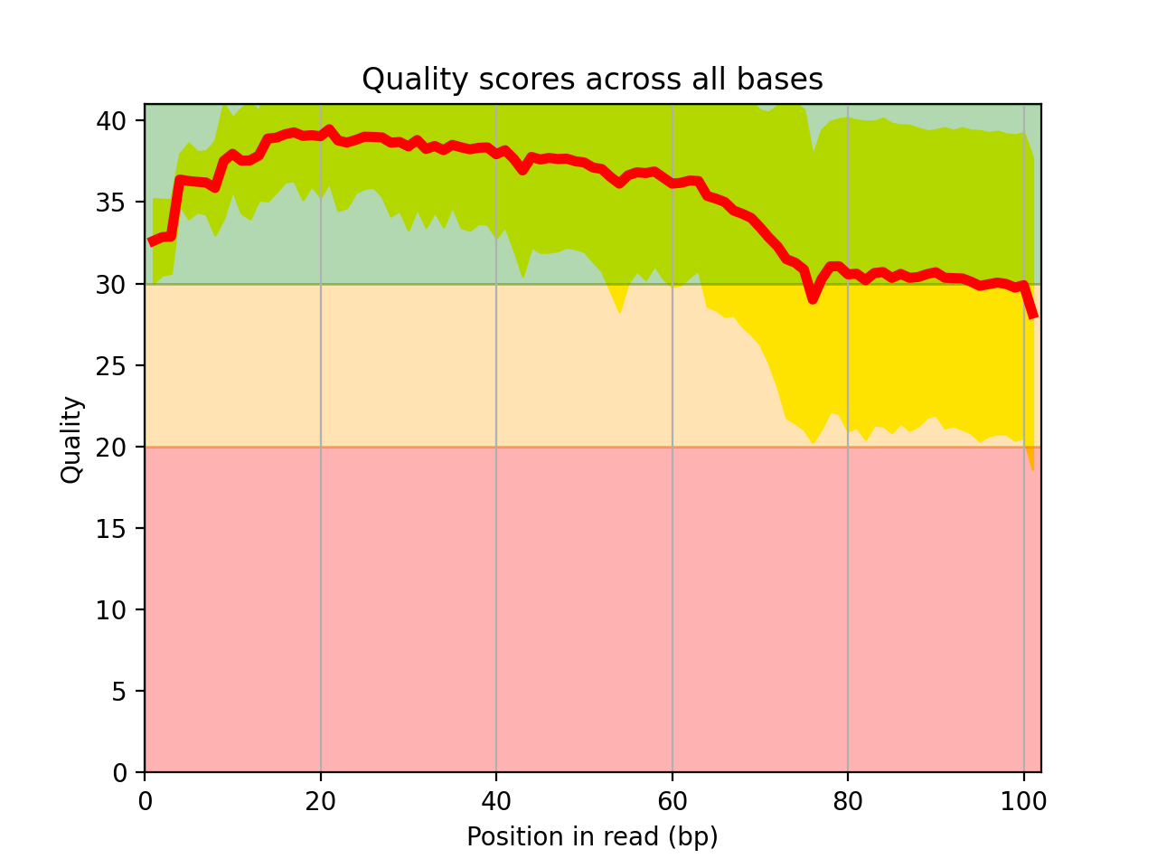
boxplot_quality(hold=False, ax=None)

Boxplot quality

Same plots as in FastQC that is average quality for all bases. In addition a 1 sigma error enveloppe is shown (yellow).

Background separate zone of good, average and bad quality (arbitrary).

get_actg_content()

get_stats()

histogram_gc_content()

Plot histogram of GC content

from sequana import sequana_data
from sequana import FastQC
filename  = sequana_data("test.fastq", "doc")
qc = FastQC(filename)
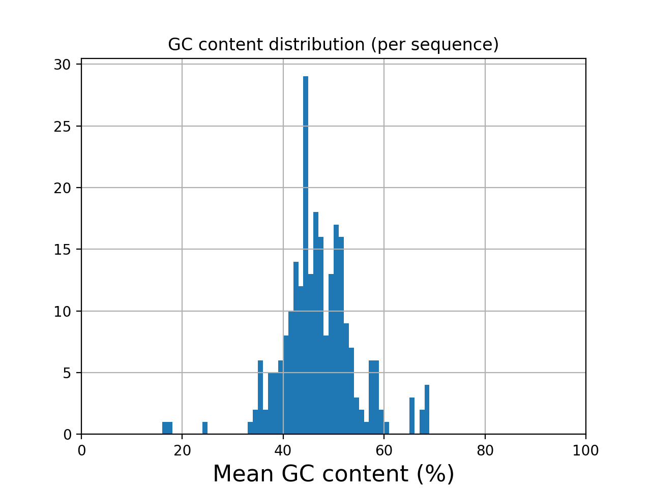
qc.histogram_gc_content()

(Source code, png, hires.png, pdf)

histogram_sequence_lengths(logy=True)

Histogram sequence lengths

from sequana import sequana_data
from sequana import FastQC
filename  = sequana_data("test.fastq", "doc")
qc = FastQC(filename)
qc.histogram_sequence_lengths()

(Source code, png, hires.png, pdf)

plot_acgt_content(stacked=False)

Plot histogram of GC content

from sequana import sequana_data
from sequana import FastQC
filename  = sequana_data("test.fastq", "doc")
qc = FastQC(filename)
qc.plot_acgt_content()

(Source code, png, hires.png, pdf)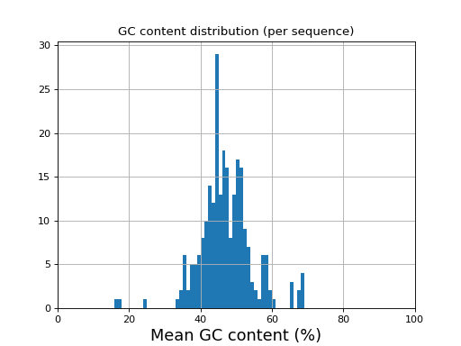

class Identifier(identifier, version='unknown')

Class to interpret Read's identifier

Warning

Implemented for Illumina 1.8+ and 1.4 . Other cases will simply stored the identifier without interpretation

>>> from sequana import Identifier
>>> ident = Identifier('@EAS139:136:FC706VJ:2:2104:15343:197393 1:Y:18:ATCACG')
>>> ident.info['x_coordinate']
'2'

Currently, the following identifiers will be recognised automatically:

Illumina_1_4:

An example is

@HWUSI-EAS100R:6:73:941:1973#0/1

Illumina_1_8:

An example is:

@EAS139:136:FC706VJ:2:2104:15343:197393 1:Y:18:ATCACG

Other that could be implemented are NCBI

@FSRRS4401BE7HA [length=395] [gc=36.46] [flows=800] [phred_min=0]                                            [phred_max=40] [trimmed_length=95]

Information can also be found here http://support.illumina.com/help/SequencingAnalysisWorkflow/Content/Vault/Informatics/Sequencing_Analysis/CASAVA/swSEQ_mCA_FASTQFiles.htm

is_fastq(filename)

class FastqSplitter(filename: str | Path)

by_part(n_parts: int, pattern: str, gzip_output: bool = False, buffer_size: int = 10000)

Split FASTQ into N parts with approximate read counting.

by_size(reads_per_chunk: int, pattern: str, gzip_output: bool = False, buffer_size: int = 10000)

Split FASTQ into chunks of N reads with file-based progress.

get_nreads()

This is a MultiQC plugin re-used temporarely here

class FastQC

A temporary class to manipulate fastqc statistics

This class can also read the output of Falco. Note, however, that falco has txt file instead of zip file.

plot_sequence_quality(max_score=40, ax=None)

read_sample(filename, s_name)

reads the fastqc stats

Parameters:

• filename

• s_name -- sample name.

This method was copied from multiqc.modules.fastqc.fastqc modules as a temporary hack to read the sample data.

BED / wig / mpileup

class BED(filename)

a structure to read and manipulate BED files (12-column file)

columns are defined as chromosome name, start and end, gene_name, score, strand, CDS start and end, blcok count, block sizes, block starts:

get_CDS_exons()

Extract CDS from input BED file.

get_exons()

Extract exon regions from input BED file.

Uses the first (chromosome name), second (chromosome start), 11th and 12th columns (exon start and size) of a 12-columns BED file.

from sequana import sequana_data
from sequana import BED
b = BED(sequana_data("hg38_chr18.bed"))
b.get_exons()

get_transcript_ranges()

Extract transcript from input BED file.

yield_wig_by_chromosome(filename)

Given a wig file such as:

variableStep chrom=1 step=1
9315 723.0
9316 723.0

you can read it using:

for chrom, entries in yield_wig_by_chromosome("example.wig"):
    print(f"Chromosome: {chrom}, {len(entries)} entries")
    print(entries[:3])

Tools to manipulate output of mpileup software

class MPileup(filename, reference, progress=True)

http://www.htslib.org/doc/samtools-mpileup.html

reference must be a string of nucleotides.

property df

get_mutation()

get_total_errors(nucs=['A', 'C', 'G', 'T'], include_deletions=False, include_Ns=False)

plot_mutation_matrix(x1=0, x2=None, vmin=0, vmax=None, cmap='hot_r')

plot_stack_bars(include_deletions=False, ec='k')

Plot error on A, C, G, T as a bar stacked plot.

plot_total_errors(nucs, include_deletions=False, include_Ns=False)

set_GC_to_AT_mutations()

Compute the mutation errors GC->AT

Here, we only consider mutation G->A, G->T, C->A, C->T. We sum the ->A an ->T errors. So, if the reference is A or T the errors is zeros.

GFF / GTF / GenBank / GFA

class GFF3(filename, skip_types=['biological_region'], light=False)

Read a GFF file, version 3

See also

The-Sequence-Ontology/Specifications

g = GFF3(filename)
# first call is slow
g.df
# print info about the different feature types
g.features
# prints info about duplicated attributes:
g.get_duplicated_attributes_per_genetic_type(self)

On eukaryotes, the reading and processing of the GFF may take a while. On prokaryotes, it should be pretty fast (a few seconds). To speed up the eukaryotes case, we skip the processing biological_regions (50% of the data in mouse).

You can do a lot with this class because your GFF is stored as a dataframe and and therefore be easily processed.

Sometimes, CDS are missing:

g = GFF3()
g.add_CDS_and_mRNA("test.gff")

Initialise a GFF3 reader.

Parameters:

• filename (str) -- path to the GFF3 file to read.

• skip_types (list) -- list of feature types to skip while reading. Defaults to ["biological_region"] which speeds up parsing of large mammalian GFF files.

Raises:

IOError -- if filename does not exist.

add_CDS_and_mRNA(output, gene_ID='gene_id')

Rewrite the GFF file adding synthetic mRNA and CDS entries for every gene.

Some annotation files (e.g. for bacteria or simple eukaryotes) contain only gene features without the corresponding mRNA/CDS children required by certain downstream tools. This method reads the source GFF line by line and, for every gene feature, emits the original gene line followed by a synthetic mRNA line and a synthetic CDS line sharing the same coordinates.

Parameters:

• output (str) -- path to the output GFF file.

• gene_ID (str) -- attribute key used to retrieve the gene identifier. Defaults to "gene_id".

add_directon_index()

Assign each gene its positional index within its directon.

For each gene, sets its ordinal position inside the directon it belongs to (assuming the GFF is sorted by chromosome and start coordinate).

Note

Not yet implemented; this method is a stub reserved for a future feature.

add_intergenic_regions()

Append intergenic regions to the internal dataframe.

Calls get_intergenic_regions() and concatenates the result with the existing annotation dataframe. Subsequent calls are no-ops (the operation is only performed once).

add_regions_and_save_gff(filename)

add missing region from the sequence-region found in the header.

clean_gff_line_special_characters(text)

Simple leaner of gff lines that may contain special characters

cluster_names_to_bed()

Identify cluster and output results in BED file

property contig_names

property df

Build and cache a pandas.DataFrame from the GFF3 file.

The dataframe contains one row per GFF3 record. Column names match the nine standard GFF3 fields (seqid, source, genetic_type, start, stop, score, strand, phase, attributes) plus one column per attribute key found in the file.

The result is cached so subsequent accesses are instantaneous.

directon_to_bed(output='directons.bed', colors={'+': '255,0,0', '-': '0,0,255'})

Write directon information to a BED9 file.

Each directon is written as one line in the output BED file with colour-coding by strand (red for +, blue for - by default).

Parameters:

• output (str) -- path for the output BED file. Defaults to "directons.bed".

• colors (dict) -- mapping from strand symbol to RGB colour string. Defaults to {"+": "255,0,0", "-": "0,0,255"}.

property directons

Compute directons: groups of consecutive genes sharing the same strand.

A directon is a maximal set of adjacent genes transcribed from the same strand. The method groups the annotation dataframe by chromosome, detects strand changes to assign each gene to a directon, then aggregates per-directon statistics (start, stop, number of genes).

The result is cached; subsequent calls return the cached value.

Returns:

DataFrame with columns seqid, strand, directon_id, start, stop, directon_length, and directon_name.

Return type:

pandas.DataFrame

property features

Extract unique GFF feature types

This is equivalent to awk '{print $3}' | sort | uniq to extract unique GFF types. No sanity check, this is suppose to be fast.

Less than a few seconds for mammals.

get_PTU()

Compute Polycistronic Transcription Units (PTUs).

PTUs are contiguous groups of genes transcribed from the same strand. tRNA and rRNA genes are excluded before computing directons (groups of genes with the same strand orientation).

Returns:

DataFrame with columns chromosome, start, stop, strand, and length (number of genes in the PTU).

Return type:

pandas.DataFrame

get_attributes(feature=None)

get_duplicated_attributes_per_genetic_type()

Report duplicated attribute values for each feature type.

Iterates over all feature types found in the GFF file and, for each attribute column, counts how many values appear more than once. The counts are printed to stdout and returned as a pandas.DataFrame whose columns are feature types and whose rows are attribute names.

Returns:

DataFrame with feature types as columns and attribute names as rows; each cell contains the number of duplicated values.

Return type:

pandas.DataFrame

get_duplicated_attributes_per_genetic_type2()

get_features_dict()

Format feature dict for sequana_coverage.

get_intergenic_regions()

Compute intergenic regions between consecutive genes on each chromosome.

For every chromosome present in the GFF, gaps between consecutive gene features (sorted by start position) are returned as a pandas.DataFrame. Each row represents one intergenic region and contains the columns seqid, start, stop, strand, attributes, source, genetic_type, score, and phase.

Returns:

DataFrame of intergenic regions.

Return type:

pandas.DataFrame

get_seqid2size()

Return a mapping from sequence identifiers to their sizes.

Sizes are read from region features in the GFF file (the stop coordinate of a region record is used as the chromosome/contig size).

Returns:

dict mapping sequence id strings to integer sizes.

Return type:

dict

get_simplify_dataframe()

Method to simplify the gff and keep only the most informative features.

is_tRNA_or_ribosomal(x)

Return True if x is not a tRNA or ribosomal RNA name.

Despite the function name, this method is intended as a boolean keep predicate: it returns True for genes that should be retained (i.e. non-tRNA, non-rRNA genes) and False for genes that should be removed (tRNA or rRNA).

Used internally to filter out tRNA and rRNA genes when computing Polycistronic Transcription Units (PTUs).

Parameters:

x -- gene name or annotation string to test.

Returns:

False if x matches a tRNA or rRNA pattern ("tRNA-", "28S", "5.8S", "18S", "5S" prefix, or exact "tRNA"), True otherwise.

Return type:

bool

read()

Read annotations one by one creating a generator

read_and_save_selected_features(outfile, features=['gene'])

Stream the GFF file and write only the requested feature types.

Unlike save_gff_filtered(), this method does not load the whole file into memory; it reads and filters line by line, making it suitable for very large GFF files.

Parameters:

• outfile (str) -- path of the output GFF file.

• features (list) -- feature types to keep. Defaults to ["gene"].

save_annotation_to_csv(filename='annotations.csv')

Save the GFF annotation dataframe to a CSV file.

Parameters:

filename (str) -- path to the output CSV file. Defaults to "annotations.csv".

save_as_gff(filename, sortby=['seqid', 'start', 'stop', 'genetic_type'])

Write the (possibly modified) annotation back to a GFF3 file.

The header comment lines from the original file are preserved. Records are sorted according to sortby using natural sort order so that chromosome identifiers like chr2 sort before chr10.

Parameters:

• filename (str) -- path to the output GFF file.

• sortby (list) -- list of column names used for sorting. Defaults to ["seqid", "start", "stop", "genetic_type"].

save_gff_filtered("test.gff", features=['misc_RNA', 'rRNA'], replace_seqid='locus_tag')

search(pattern)

Search all columns of the annotation dataframe for a pattern.

Converts every cell to a string and returns all rows where at least one column contains pattern as a substring.

Parameters:

pattern -- search term (converted to str internally).

Returns:

filtered copy of the annotation dataframe.

Return type:

pandas.DataFrame

to_bed(output_filename, attribute_name, features=['gene'])

Experimental export to BED format to be used with rseqc scripts

Parameters:

attribute_name (str) -- the attribute_name name to be found in the GFF attributes

to_fasta(ref_fasta, fasta_out, features=['gene'], identifier='ID')

From a genomic FASTA file ref_fasta, extract regions stored in the gff. Export the corresponding regions to a FASTA file fasta_out.

Parameters:

• ref_fasta -- path to genomic FASTA file to extract rRNA regions from.

• fasta_out -- path to FASTA file where rRNA regions will be exported to.

to_gtf(output_filename='test.gtf', mapper={'ID': '{}_id'})

Convert the GFF3 file to GTF format (experimental).

Reads the source GFF3 file line by line and rewrites each record in GTF format. Attribute keys are renamed according to mapper which maps GFF3 attribute names to GTF attribute name templates; the {} placeholder in the template is replaced with the feature type.

Parameters:

• output_filename (str) -- path for the output GTF file. Defaults to "test.gtf".

• mapper (dict) -- mapping from GFF3 attribute keys to GTF attribute name templates. Defaults to {"ID": "{}_id"} which converts the GFF3 ID attribute to e.g. gene_id or exon_id.

Note

This method is experimental and is used by the Sequana RNA-seq pipeline to convert input GFF files to GTF format for RNA-seqc.

to_pep(ref_fasta, fasta_out)

Extract CDS, convert to proteines and save in file

transcript_to_gene_mapping(feature='all', attribute='transcript_id')

Parameters:

• feature -- not used yet

• attribute -- the attribute to be usde. should be transcript_id for salmon compatability but could use soething different.

class GenBank(filename, skip_types=['biological_region'])

This class reads a Genbank file

This is kept for back compatibility but most code in Sequana will rely on sequana.gff3.GFF3 instead. So please, transform your genbank to GFF3 format if possible.

gg = GenBank()
gg.get_types()

extract_fasta(fastafile, features=['rRNA'])

property features

genbank_features_parser()

Return dictionary with features contains inside a genbank file.

Parameters:

input_filename (str) -- genbank formated file

get_types()

Utilities for GTF files

class GTFFixer(filename)

Some GTF have syntax issues. This class should fix some of them

With exons, we want to have unique IDs.

We append the transcrpt version and ID to the exon ID

fix(output)

class GFA(filename)

read()

Utilities to manipulate FastA files

class FastaGFFCorrection(fasta_file, vcf_file)

Class to correct FastA reference and its GFF given a set of variants

::

f = FastaGFFCorrection("input.fa", "input.vcf") f.fix_and_save_fasta("new.fa") f.fix_and_save_gff("new.fa", "input.gff3", "new.gff3")

You must call save_fasta() before save_gff() to compute the shifts of positions found in the VCF file.

The GFF corrections are made on the start and stop positions of all features found in the GFF. In addition, gene and CDS start and stop positions are also corrected for the change of start/stop codon implied by the variants.

find_start_codon_position(sequence, position, strand)

return position of start codon

fix_and_save_fasta(outfile)

We consider that the VCF file contains variants that have already been filtered.

Todo

handle multiple-variants at a given position

fix_and_save_gff(gff_infile, fasta_corrected, gff_outfile, maxshift=8000)

Corrects the start/stop codons of input GFF given corrected fasta

You must call fix_and_save_fasta() first.

Todo

multiple contig is not yet implemented

get_all_start_codons(fasta, gff, chr_name, strand, feature='CDS')

On strand +, start codon are ATG, TTG, GTG On strand -, start codon (from 3-5 prime) are CAT, CAA, CAC (reverse complement of start codon on strand+).

get_all_stop_codons(fasta, gff, chr_name, strand, feature='CDS')

On strand +, stop codons are TAG, TGA, TAA On strand -, stop codons (from 3-5 prime) are TTA, TCA, CTA (reverse complement of start codon on strand+).

class Aragorn

# Example usage:

file_path = 'aragorn_output.txt'  # Replace with the path to your Aragorn output file
parsed_results = parse_aragorn_output(file_path)

for result in parsed_results:
   print(result)

parse_aragorn_output(file_path)

run(fasta_file, output='aragorn.txt')

class CMSearchParser(filename)

class PAFReader(filename)

class RAGTAG(filename)

class RFAMSplitter(filename)

extract(accession_list, outfile)

split_records(maxchunks=10, output='rfam_{chunk}.cm')

class RNAmmer(filename)

input is the GFF file from rnammer that is in gff2 format.

##gff-version2 ##source-version RNAmmer-1.2 ##date 2024-09-09 ##Type DNA # seqname source feature start end score +/- frame attribute # --------------------------------------------------------------------------------------------------------- 11 RNAmmer-1.2 rRNA 394875 394989 59.3 + . 8s_rRNA 21 RNAmmer-1.2 rRNA 605807 605921 60.0 + . 8s_rRNA 9 RNAmmer-1.2 rRNA 417374 417488 63.6 + . 8s_rRNA 21 RNAmmer-1.2 rRNA 319355 319469 61.1 - . 8s_rRNA

to_gff3(filename)

VCF

Python script to filter a VCF file

compute_fisher_strand_filter(record)

Fisher strand filter (FS).

Sites where the numbers of reference/non-reference reads are highly correlated with the strands of the reads. Counting the number of reference reads on the forward strand and on the reverse strand, and the number of alternate reads on the forward and reverse strand should be equivalent. With these four numbers, we construct a 2 x 2 contingency table and used the P-value from a Fisher’s exact test to evaluate the correlation.

from sequana import freebayes_vcf_filter v = freebayes_vcf_filter.VCF_freebayes("data/JB409847.vcf") r = next(v) compute_fisher_strand_filter(r)

If the pvalue is less than 0.05 we should reject the variant since the alternate and reference do not behave in the same way. Typically found if the alternate has a poor strand balance. Used with care if frequency of alternate or reference is low or deth of coverage is low.

Note

fisher terst with two-sided hypothesis

compute_frequency(record)

Compute frequency of alternate allele.

alt_freq = Count Alternate Allele / Depth

Parameters:

record -- variant record

compute_strand_balance(record)

Compute strand balance of alternate allele include in [0,0.5]. strand_bal = Alt Forward / (Alt Forward + Alt Reverse)

Parameters:

record -- variant record

FYI: in freebayes, the allele balance (reported under AB), strand bias counts (SRF, SRR, SAF, SAR) and bias estimate (SAP) can be used as well for filtering. Here, we use the strand balance computed as SAF / (SAF + SAR)

strand_ratio(number1, number2)

Compute ratio between two number. Return result between [0:0.5].

class FilteredVariantFile(variants, fb_vcf)

Variants filtered with VCF_freebayes.

Class kept for back compatiblity in wrappers and variant_calling pipeline

constructor

Parameters:

• variants (list) -- list of variants record.

• fb_vcf (VCF_freebayes) -- class parent.

property df

Get the data frame.

to_csv(output_filename, info_field=False)

Write DataFrame in CSV format.

Params str output_filename:

output CSV filename.

to_vcf(output_filename)

Write VCF file in VCF format.

Params str output_filename:

output VCF filename.

property variants

Get the variant list.

property vcf

Get the VCF_freebayes object.

class VariantFile(filename, progress=False, keep_polymorphic=True)

Reads a BCF or VCF or GZIPPED VCF

v = VariantFile()

You can access to a list of all variants (unchanged from pysam) using:

vlist = v.variants

you may transform a variant into a dictionary that contains a subset of most important information including SNPeff annotation (if available) using:

v._variant_to_dict(vlist[0])

A dataframe of all variants processed with this _variant_to_dict function is provided as an attribute:

v.df

Samples and contigs/chromosomes are available also as attributes:

v.samples
v.contigs
v.chromosomes # a synomym of v.contigs

There is a set of parameter to filter variants. To apply it, use the filter_vcf function.

fvcf = v.filter_vcf()

barplot()

property chromosomes

property contigs

property df

filter_vcf(filter_dict=None)

Filter variants in the VCF file.

Parameters:

filter_dict (dict) -- dictionary of filters. It updates the attribute VCF_freebayes.filter_params

Return Filtered_freebayes object.

get_variant_type()

hist_score(bins=200, min_score=1)

Histogram of Quality score

property is_joint

manhattan_plot(chrom_name=None, bins=200, types=['ins', 'del', 'mnp', 'snp', 'complex', 'INS', 'DEL'])

pieplot()

plot_frequency()

property samples

to_vcf(output_filename)

Write VCF file in VCF format.

Params str output_filename:

output VCF filename.

property variants

apply_variants(fasta_path, vcf_path, output_fasta)

Other formats

class PfamDomtblout(filepath)

parser for the output of hmmscan (domtblout format)

hmmscan --cpu 8 --domtblout pfam.domtblout Pfam-A.hmm temp.faa > pfam.hmmscan.txt

annotate_gff(augustus_gff, out_gff, key='pfam')

add pfam+description into original GFF file

read()

to_gff(output_file, augustus_gff=None, best_hit=True)

class MGI(filename)

boxplot_quality(color_line='r', bgcolor='grey', color='yellow', lw=4, hold=False, ax=None)

plot_acgt()

IEM class

class IEM(filename)

class SampleSheet(filename)

Reader and validator of Illumina samplesheets

The Illumina samplesheet reader and validator verifies the correctness of the sections in the samplesheet, which are not case-sensitive and are enclosed within square brackets.

Following the closing bracket, no additional characters are permitted, except for commas and the end-of-line marker. For instance [Data]a prevents the [Data] section from being correctly processed.

The sections then consist of key-value pairs represented as records, with each line consisting of precisely two fields.

An optional [Settings] section can contain key-value pairs, and the [Reads] section specifies the number of cycles per read, which is exclusively required for MiSeq.

The [Data] section, which is a table similar to CSV format, is optional. However, without [Data] section all reads are sent to a single 'undetermined' output file. Sample_ID is highly recommended.

Example of typical Data section to be used with bcl2fastq:

[Header]

[Data]
Sample_ID,Sample_Name,I7_Index_ID,index,I5_INdex_ID,index2
A10001,Sample_A,D701,AATACTCG,D501,TATAGCCT
A10002,Sample_B,D702,TCCGGAGA,D501,TATAGCCT
A10003,Sample_C,D703,CGCTCATT,D501,TATAGCCT
A10004,Sample_D,D704,GAGATTCC,D501,TATAGCCT

Important: altough we have upper case names as specified in the Illumina specs, the bcl2fastq does not care about the upper case. This is not intuitive since IEM produces keys with upper and lower case names similarly to the specs.

Sequana Standalone

The standalone application sequana contains a subcommand based on this class:

sequana samplesheet

that can be used to check the correctness of a samplesheet:

sequana samplesheet --check SampleSheet.csv

References:

illumina specifications 970-2017-004.pdf

checker()

property df

Returns the [Data] section

expected_data_headers = {'PE': [], 'SE': []}

expected_headers_fields = ['IEMFileVersion', 'Investigator Name', 'Instrument Type', 'Experiment Name', 'Date', 'Workflow', 'Application', 'Assay', 'Description', 'Chemistry', 'Index Adapters']

property header

property index_adapters

returns index adapters

property instrument

returns instrument name

quick_fix(output_filename)

Fix sample sheet

Tyical error is when users save the samplesheet as CSV file in excel. This may add trailing ; characters at the end of section, which raises error in bcl2fastq.

property samples

returns the sample identifiers as a list

property settings

to_fasta(adapter_name='')

Extract adapters from [Adapter] section and print them as a fasta file

validate()

This method checks whether the sample sheet is correctly formatted

Checks for:

• presence of ; at the end of lines indicated an edition with excel that wrongly transformed the data into a pure CSV file

• inconsistent numbers of columns in the [DATA] section, which must be CSV-like section

• Extra lines at the end are ignored

• special characters are forbidden except - and _

• checks for Sample_ID column uniqueness

• checks for index uniqueness (if single index)

• checks for combo of dual indices uniqueness

• checks that sample names are unique

and raise a SystemExit error on the first found error.

property version

return the version of the IEM file

class Cigar(cigarstring: str)

A class to handle CIGAR strings from BAM files.

>>> from sequana.cigar import Cigar
>>> c = Cigar("2S30M1I")
>>> len(c)
33

>>> c = Cigar("1S1S1S1S")
>>> c.compress()
>>> c.cigarstring
'4S'

Possible CIGAR types are:

• "M" : alignment match

• "I" : insertion to the reference

• "D" : deletion from the reference

• "N" : skipped region from the reference

• "S" : soft clipping (clipped sequence present in seq)

• "H" : hard clipping (sequence NOT present)

• "P" : padding (silent deletion from padded reference)

• "=" : sequence match

• "X" : sequence mismatched

• "B" : back (rare) (could be also NM ?)

!!! BWA MEM get_cigar_stats returns list with 11 items Last item is !!! what is the difference between M and = ??? Last item is I + S + X !!! dans BWA, mismatch (X) not provided... should be deduced from last item - I - S

Note

the length of the query sequence based on the CIGAR is calculated by adding the M, I, S, =, or X and other operations are ignored. source: https://stackoverflow.com/questions/39710796/infer-the-length-of-a-sequence-using-the-cigar/39812985#39812985

Reference:

samtools/htslib

Constructor

Parameters:

cigarstring (str) -- the CIGAR string.

Note

the input CIGAR string validity is not checked. If an unknown type is found, it is ignored generally. For instance, the length of 1S100Y is 1 since Y is not correct.

as_dict()

Return cigar types and their count

Returns:

dictionary

Note that repeated types are added:

>>> c = Cigar('1S2M1S')
>>> c.as_dict()
{"S":2,"M":2}

as_sequence()

as_tuple()

Decompose the cigar string into tuples keeping track of repeated types

Returns:

tuple

>>> from sequana import Cigar
>>> c = Cigar("1S2M1S")
>>> c.as_tuple()
(('S', 1), ('M', 2), ('S', 1))

property cigarstring

compress()

1S1S should become 2S. inplace modification

get_query_length() → int

Return length consumed by the query (read).

get_reference_length() → int

Return length consumed by the reference.

pattern = re.compile('(\\d+)([A-Za-z])?')

stats()

Returns number of occurence for each type found in types

>>> c = Cigar("1S2M1S")
>>> c.stats()
[2, 0, 0, 0, 2, 0, 0, 0, 0, 0]

types = 'MIDNSHP=XB'

fetch_clip(chrom, start, cigar)

fetch_deletion(chrom, start, cigar)

fetch_exon(chrom, start, cigar)

fetch_insertion(chrom, start, cigar)

fetch_intron(chrom, start, cigar)

Sniffer

sniffer(filename)