13. References (stats)

13.1. Statistical tools

Statistical tools

evenness(data)

Return Evenness of the coverage

Reference:

Konrad Oexle, Journal of Human Genetics 2016, Evaulation of the evenness score in NGS.

work before or after normalisation but lead to different results.

moving_average(data, n)

Compute moving average

Parameters:

n -- window's size (odd or even).

>>> from sequana.stats import moving_average as ma
>>> ma([1,1,1,1,3,3,3,3], 4)
array([ 1. ,  1.5,  2. ,  2.5,  3. ])

Note

the final vector does not have the same size as the input vector.

runmean(data, n)

Akaike and other criteria

AIC(L, k, logL=False)

Return Akaike information criterion (AIC)

Parameters:

• L (float) -- maximised value of the likelihood function

• k (int) -- number of parameters

• logL (bool) -- L is the log likelihood.

Suppose that we have a statistical model of some data, from which we computed its likelihood function and let be the number of parameters in the model (i.e. degrees of freedom). Then the AIC value is: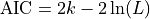

Given a set of candidate models for the data, the preferred model is the one with the minimum AIC value. Hence AIC rewards goodness of fit (as assessed by the likelihood function), but it also includes a penalty that is an increasing function of the number of estimated parameters. The penalty discourages overfitting.

Suppose that there are R candidate models AIC1, AIC2, AIC3, AICR. Let AICmin be the minimum of those values. Then, exp((AICmin - AICi)/2) can be interpreted as the relative probability that the ith model minimizes the (estimated) information loss.

Suppose that there are three candidate models, whose AIC values are 100, 102, and 110. Then the second model is exp((100 - 102)/2) = 0.368 times as probable as the first model to minimize the information loss. Similarly, the third model is exp((100 - 110)/2) = 0.007 times as probable as the first model, which can therefore be discarded.

With the remaining two models, we can (1) gather more data, (2) conclude that the data is insufficient to support selecting one model from among the first two (3) take a weighted average of the first two models, with weights 1 and 0.368.

The quantity exp((AIC_{min} - AIC_i)/2) is the relative likelihood of model i.

If all the models in the candidate set have the same number of parameters, then using AIC might at first appear to be very similar to using the likelihood-ratio test. There are, however, important distinctions. In particular, the likelihood-ratio test is valid only for nested models, whereas AIC (and AICc) has no such restriction.

Reference:

Burnham, K. P.; Anderson, D. R. (2002), Model Selection and Multimodel Inference: A Practical Information-Theoretic Approach (2nd ed.), Springer-Verlag, ISBN 0-387-95364-7.

AICc(L, k, n, logL=False)

AICc criteria

Parameters:

• L (float) -- maximised value of the likelihood function

• k (int) -- number of parameters

• n (int) -- sample size

• logL (bool) -- L is the log likelihood.

AIC with a correction for finite sample sizes. The formula for AICc depends upon the statistical model. Assuming that the model is univariate, linear, and has normally-distributed residuals (conditional upon regressors), the formula for AICc is as follows:

AICc is essentially AIC with a greater penalty for extra parameters. Using AIC, instead of AICc, when n is not many times larger than k2, increases the probability of selecting models that have too many parameters, i.e. of overfitting. The probability of AIC overfitting can be substantial, in some cases.

BIC(L, k, n, logL=False)

Bayesian information criterion

Parameters:

• L (float) -- maximised value of the likelihood function

• k (int) -- number of parameters

• n (int) -- sample size

• logL (bool) -- L is the log likelihood.

Given any two estimated models, the model with the lower value of BIC is the one to be preferred.

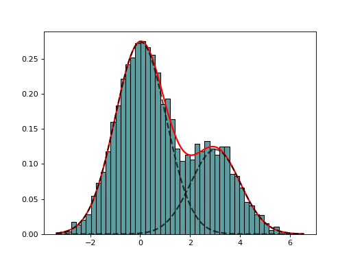
class EM(data, model=None, max_iter=100)

Expectation minimization class to estimate parameters of GMM

from sequana import mixture
from pylab import normal
data = [normal(0,1) for x in range(7000)] + [normal(3,1) for x in range(3000)]
em = mixture.EM(data)
em.estimate(k=2)
em.plot()

(Source code, png, hires.png, pdf)

constructor

Parameters:

• data --

• model -- not used. Model is the GaussianMixtureModel but could be other model.

• max_iter (int) -- max iteration for the minization

estimate(guess=None, k=2)

Parameters:

• guess (list) -- a list to provide the initial guess. Order is mu1, sigma1, pi1, mu2, ...

• k (int) -- number of models to be used.

plot(model_parameters=None, **kwargs)

Take a list of dictionnaries with models parameters to plot predicted models. If user doesn't provide parameters, the standard plot function from fitting is used.

Example:

model_parameters=[{"mu": 5, "sigma": 0.5, "pi": 1}]

class Fitting(data, k=2, method='Nelder-Mead')

Base class for EM and GaussianMixtureFitting

constructor

Parameters:

• data (list) --

• k (int) -- number of GMM to use

• method (str) -- minimization method to be used (one of scipy optimise module)

get_guess()

Random guess to initialise optimisation

property k

property model

plot(normed=True, N=1000, Xmin=None, Xmax=None, bins=50, color='red', lw=2, hist_kw={'color': '#5F9EA0', 'edgecolor': 'k'}, ax=None)

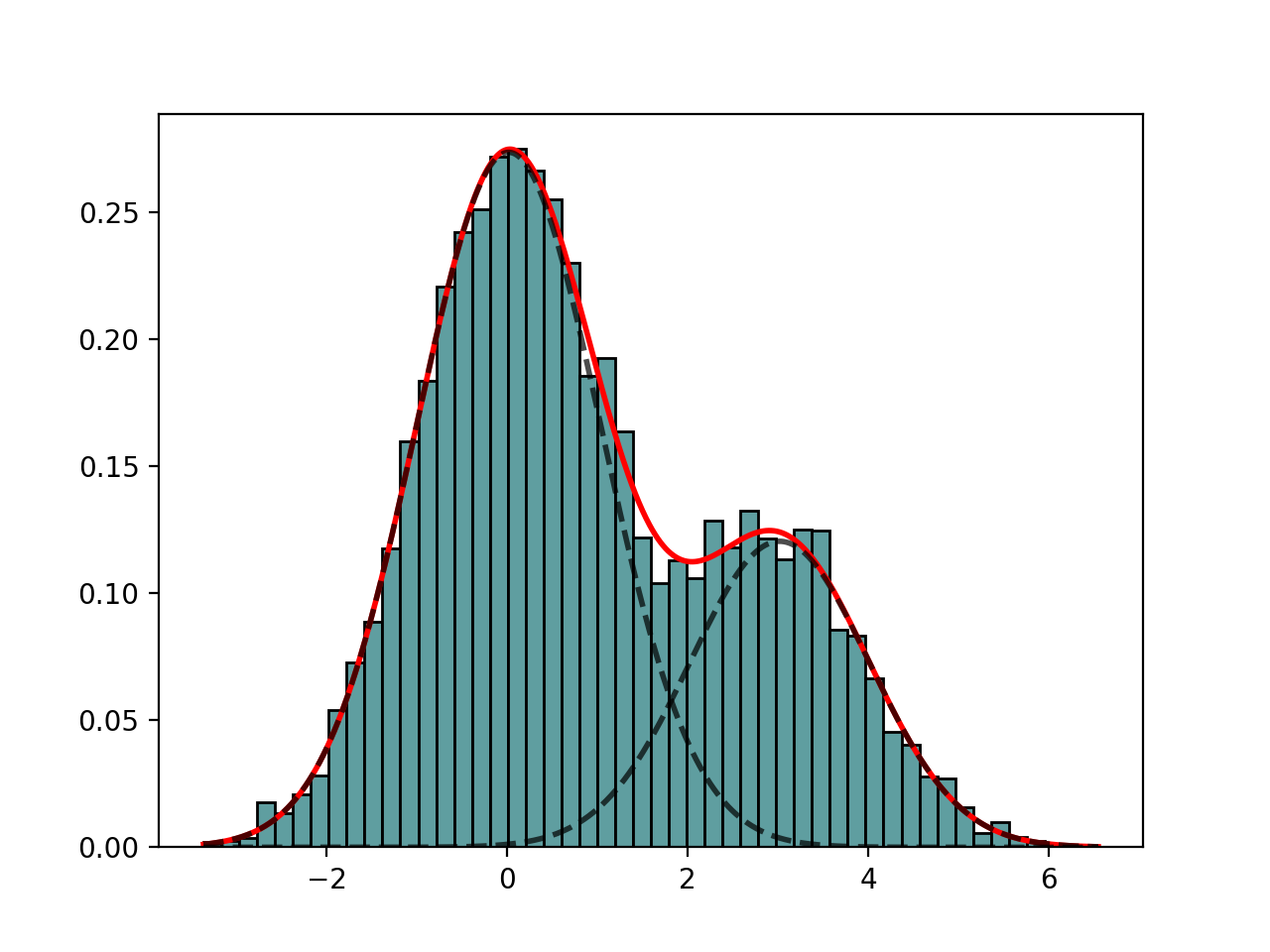
class GaussianMixtureFitting(data, k=2, method='Nelder-Mead')

GaussianMixtureFitting using scipy minization

from sequana import mixture
from pylab import normal
data = [normal(0,1) for x in range(700)] + [normal(3,1) for x in range(300)]
mf = mixture.GaussianMixtureFitting(data)
mf.estimate(k=2)
mf.plot()

(Source code, png, hires.png, pdf)

Here we use the function minimize() from scipy.optimization. The list of (currently) available minimization methods is 'Nelder-Mead' (simplex), 'Powell', 'CG', 'BFGS', 'Newton-CG',> 'Anneal', 'L-BFGS-B' (like BFGS but bounded), 'TNC', 'COBYLA', 'SLSQPG'.

estimate(guess=None, k=None, maxfev=20000.0, maxiter=1000.0, bounds=None)

guess is a list of parameters as expected by the model

guess = {'mus':[1,2], 'sigmas': [0.5, 0.5], 'pis': [0.3, 0.7] }

property method

class GaussianMixtureModel(k=2)

Gaussian Mixture Model

(Source code, png, hires.png, pdf)

log_likelihood(params, sample)

pdf(x, params, normalise=True)

Expected parameters are

params is a list of gaussian distribution ordered as mu, sigma, pi, mu2, sigma2, pi2, ...

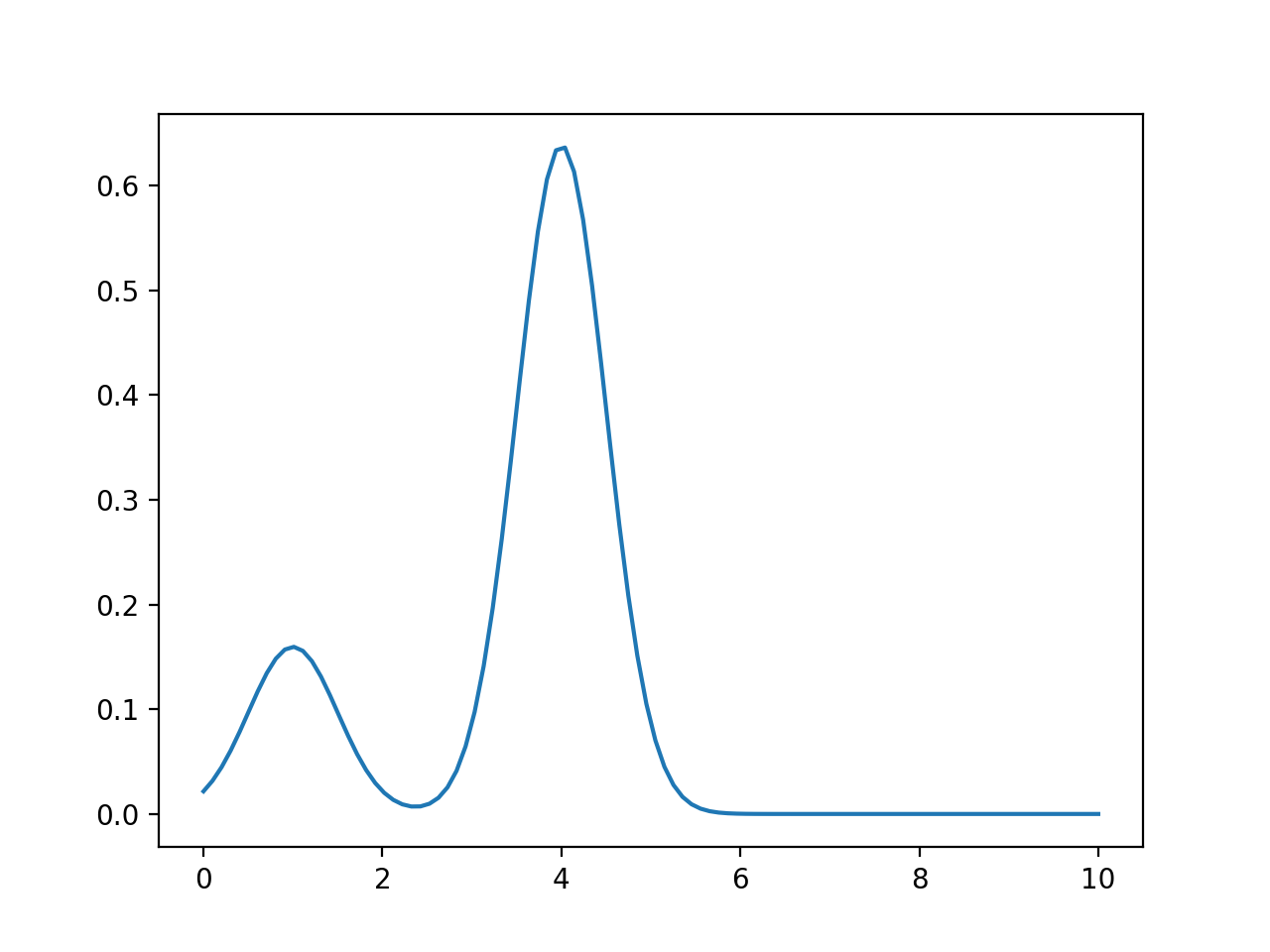
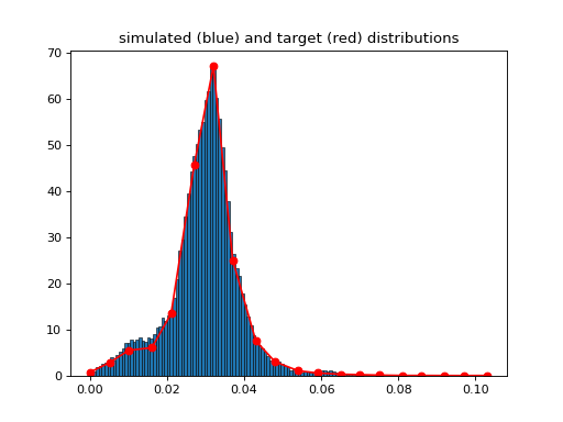
class MetropolisHasting

(Source code, png, hires.png, pdf)

property Xtarget

property Ytarget

check(bins=60)

diagnostics(bins=60, clear=True)

simulate(n=100000, burning=20000, step=None, x0=None)

Simple VST transformation

class VST

v = VST()
v.anscombe(X)

Reference: M. Makitalo and A. Foi, "Optimal inversion of the

generalized Anscombe transformation for Poisson-Gaussian noise", IEEE Trans. Image Process., doi:10.1109/TIP.2012.2202675

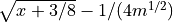
static anscombe(x)

Compute the anscombe variance stabilizing transform.

Parameters:

x -- noisy Poisson-distributed data

Returns:

data with variance approximately equal to 1.

Reference: Anscombe, F. J. (1948), "The transformation of Poisson,

binomial and negative-binomial data", Biometrika 35 (3-4): 246-254

For Poisson distribution, the mean and variance are not independent. The anscombe transform aims at transforming the data so that the variance is about 1 for large enough mean; For mean zero, the varaince is still zero. So, it transform Poisson data to approximately Gaussian data with mean

static generalized_anscombe(x, mu, sigma, gain=1.0)

Compute the generalized anscombe variance stabilizing transform

Data should be a mixture of poisson and gaussian noise.

The input signal z is assumed to follow the Poisson-Gaussian noise model:

x = gain * p + n

where gain is the camera gain and mu and sigma are the read noise mean and standard deviation. X should contain only positive values. Negative values are ignored. Biased for low counts

static inverse_anscombe(x)

Compute the inverse transform

This uses an approximation of the exact unbiased inverse. Reference: Makitalo, M., & Foi, A. (2011). A closed-form approximation of the exact unbiased inverse of the Anscombe variance-stabilizing transformation. Image Processing.