11. References

11.1. Assembly and contigs related

class BUSCO(filename='full_table_test.tsv')

Wrapper of the BUSCO output

"BUSCO provides a quantitative measures for the assessment of a genome assembly, gene set, transcriptome completeness, based on evolutionarily-informed expectations of gene content from near-universal single-copy orthologs selected from OrthoDB v9." -- BUSCO website 2017

This class reads the full report generated by BUSCO and provides some visualisation of this report. The information is stored in a dataframe df. The score can be retrieve with the attribute score in percentage in the range 0-100.

Reference:

http://busco.ezlab.org/

Note

support version 3.0.1 and new formats from v5.X

constructor

Filename:

a valid BUSCO input file (full table). See example in sequana code source (testing)

get_summary_string()

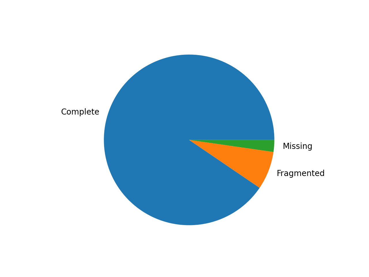
pie_plot(filename=None, hold=False)

Pie plot of the status (completed / fragment / missed)

from sequana import BUSCO, sequana_data
b = BUSCO(sequana_data("test_busco_full_table.tsv"))
b.pie_plot()

(Source code, png, hires.png, pdf)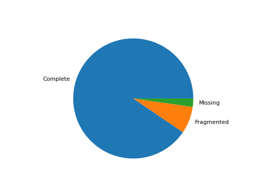

save_core_genomes(contig_file, output_fasta_file='core.fasta')

Save the core genome based on busco and assembly output

The busco file must have been generated from an input contig file. In the example below, the busco file was obtained from the data.contigs.fasta file:

from sequana import BUSCO
b = BUSCO("busco_full_table.tsv")
b.save_core_genomes("data.contigs.fasta", "core.fasta")

If a gene from the core genome is missing, the extracted gene is made of 100 N's If a gene is duplicated, only the best entry (based on the score) is kept.

If there are 130 genes in the core genomes, the output will be a multi-sequence FASTA file made of 130 sequences.

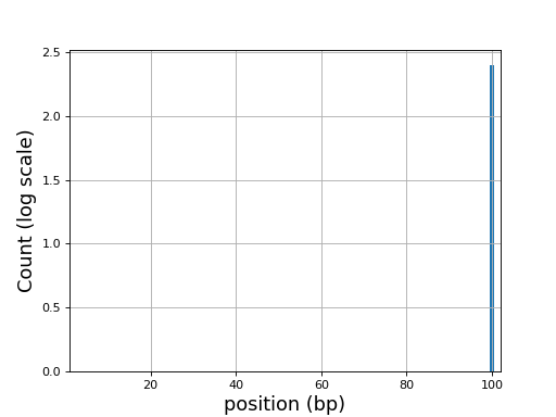
scatter_plot(filename=None, hold=False)

Scatter plot of the score versus length of each ortholog

from sequana import BUSCO, sequana_data
b = BUSCO(sequana_data("test_busco_full_table.tsv"))
b.scatter_plot()

(Source code, png, hires.png, pdf)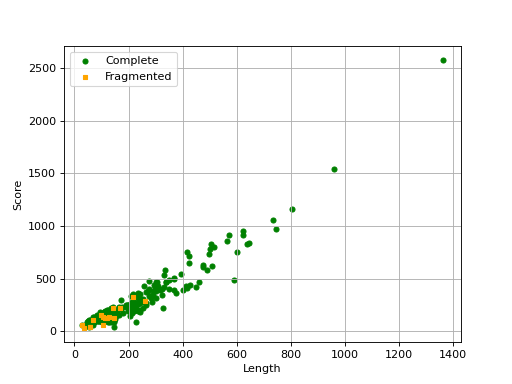

Missing are not show since there is no information about contig .

property score

summary()

Return summary information of the missing, completed, fragemented orthologs

class Contigs(filename, mode='canu')

Utilities for summarising or plotting contig information

Depending on how the FastA file was created, different types of plots can be are available. For instance, if the FastA was created with Canu, nreads and covStat information can be extracted. Therefore, plots such as plot_scatter_contig_length_vs_nreads_cov() and plot_contig_length_vs_nreads() can be used.

Constructor

Parameters:

• filename -- input FastA file

• canu -- tool that created the output file.

property df

hist_plot_contig_length(bins=40, fontsize=16, lw=1)

Plot distribution of contig lengths

Parameters:

• bin -- number of bins for the histogram

• fontsize -- fontsize for xy-labels

• lw -- width of bar contour edges

• ec -- color of bar contours

(Source code, png, hires.png, pdf)

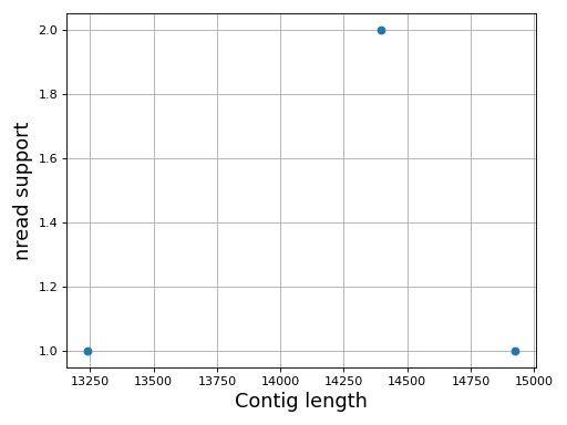
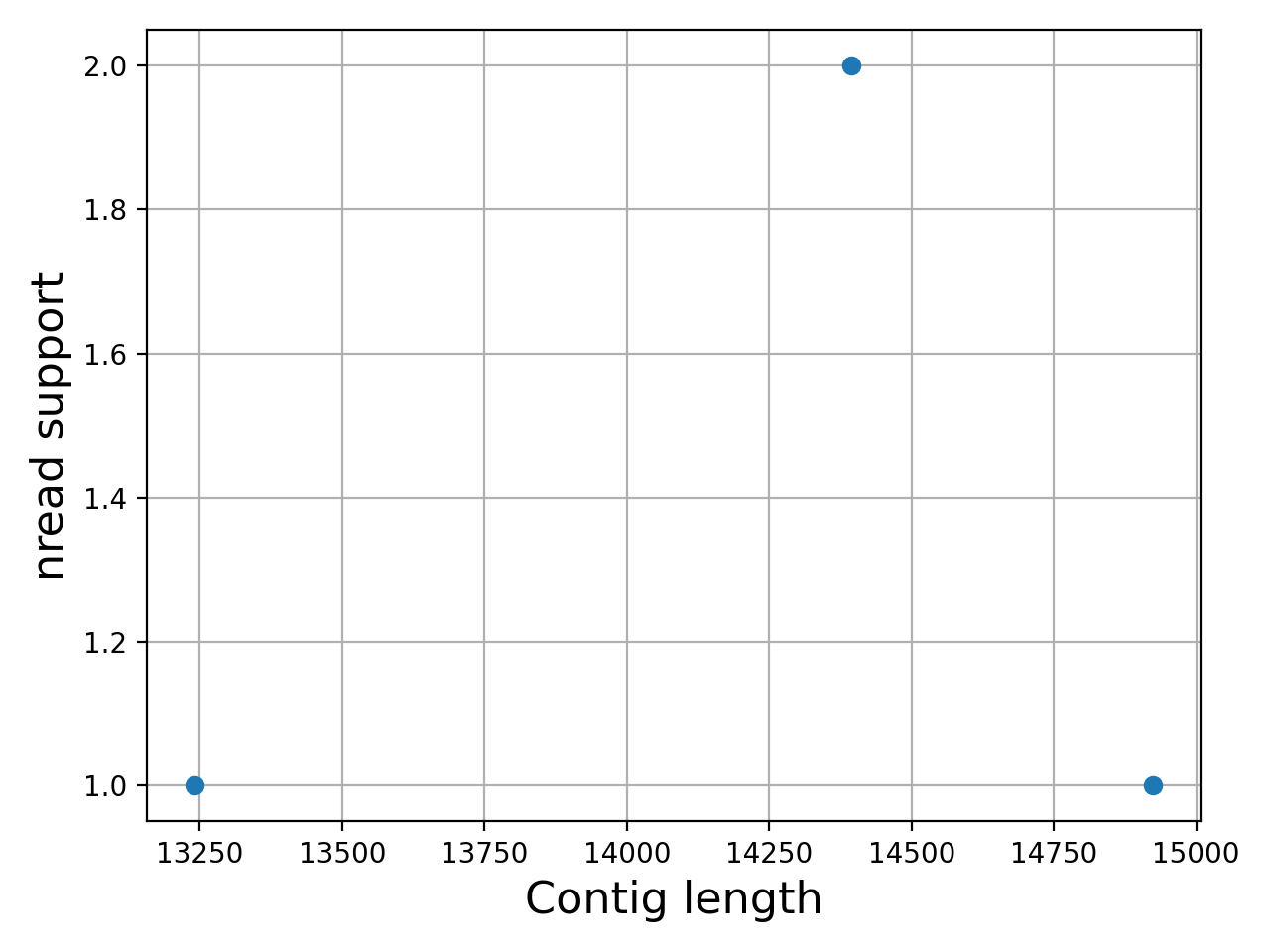
plot_contig_length_vs_nreads(fontsize=16, min_length=5000, min_nread=10, grid=True, logx=True, logy=True)

Plot contig length versus nreads

In canu, contigs have the number of reads that support them. Here, we can see whether contigs have lots of reads supported them or not.

Note

For Canu output only

(Source code, png, hires.png, pdf)

plot_scatter_contig_length_vs_nreads_cov(fontsize=16, vmin=0, vmax=50, min_nreads=20, min_length=5000, grid=True, logx=True, logy=True)

Scatter plot showing number of support reads and contig lengths

Note

only for Canu output.

(Source code)

stats()

Return N50, L50 and total cumulated length

class ContigsBase(filename)

Parent class for contigs data

Constructor

Parameters:

filename -- input file name

get_gc(window=100)

Return GC content for each contig

plot_contig_length_vs_GC(alpha=0.5)

Plot contig GC content versus contig length

(Source code, png, hires.png, pdf)

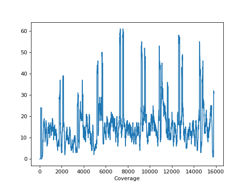
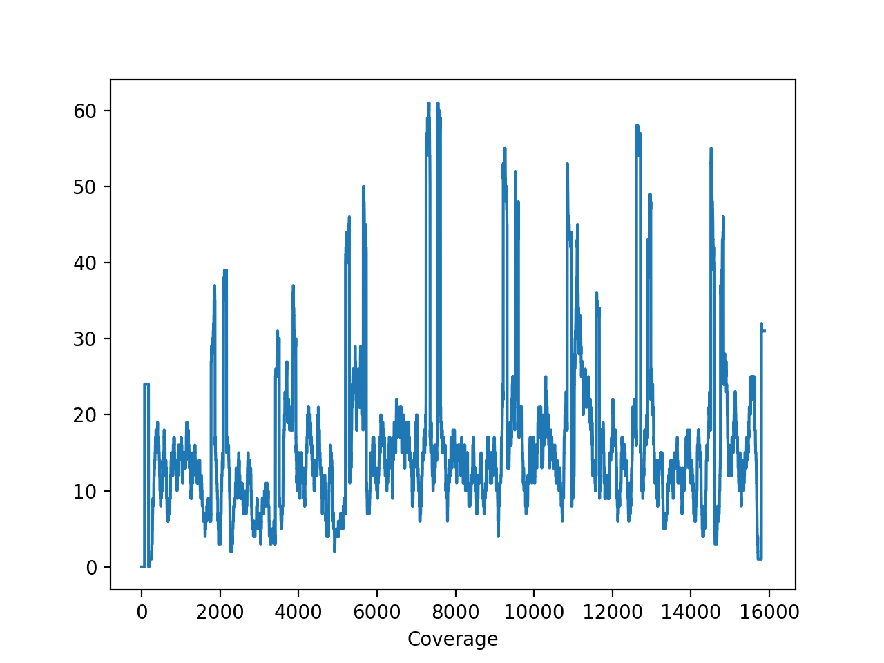
scatter_length_cov_gc(min_length=200, min_cov=10, grid=True, logy=False, logx=True)

Plot scatter length versus GC content

Parameters:

• min_length -- add vertical line to indicate possible contig length cutoff

• min_cov -- add horizontal line to indicate possible coverage contig cutff

• grid -- add grid to the plot

• logy -- set y-axis log scale

• logx -- set x-axis log scale

(Source code, png, hires.png, pdf)

11.2. BAMTOOLS related

Tools to manipulate BAM/SAM files

Alignment(alignment)	Helper class to retrieve info about Alignment
BAM(filename, *args)	BAM reader.
CRAM(filename, *args)	CRAM Reader.
MultiBAM()	Convenient structure to store several BAM files
SAM(filename, *args)	SAM Reader.
SAMFlags([value])	Utility to extract bits from a SAM flag
SAMBAMbase(filename[, mode])	Base class for SAM/BAM/CRAM data sets

Note

BAM being the compressed version of SAM files, we do not implement any functionalities related to SAM files. We strongly encourage developers to convert their SAM to BAM.

class Alignment(alignment)

Helper class to retrieve info about Alignment

Takes an alignment as read by BAM and provides a simplified version of pysam.Alignment class.

>>> from sequana.bamtools import Alignment
>>> from sequana import BAM, sequana_data
>>> b = BAM(sequana_data("test.bam"))
>>> segment = next(b)
>>> align = Alignment(segment)
>>> align.as_dict()
>>> align.FLAG
353

The original data is stored in hidden attribute _data and the following values are available as attributes or dictionary:

• QNAME: a query template name. Reads/segment having same QNAME come from the same template. A QNAME set to * indicates the information is unavailable. In a sam file, a read may occupy multiple alignment

• FLAG: combination of bitwise flags. See SAMFlags

• RNAME: reference sequence

• POS

• MAPQ: mapping quality if segment is mapped. equals -10 log10 Pr

• CIGAR: See sequana.cigar.Cigar

• RNEXT: reference sequence name of the primary alignment of the NEXT read in the template

• PNEXT: position of primary alignment

• TLEN: signed observed template length

• SEQ: segment sequence

• QUAL: ascii of base quality

constructor

Parameters:

alignment -- alignment instance from BAM

as_dict()

class BAM(filename, *args)

BAM reader. See SAMBAMbase for details

class CRAM(filename, *args)

CRAM Reader. See SAMBAMbase for details

class CS(tag)

Interpret CS tag from SAM/BAM file tag

>>> from sequana import CS
>>> CS('-a:6-g:14+g:2+c:9*ac:10-a:13-a')
{'D': 3, 'I': 2, 'M': 54, 'S': 1}

When using some mapper, CIGAR are stored in another format called CS, which also includes the substitutions. See minimap2 documentation for details.

class SAM(filename, *args)

SAM Reader. See SAMBAMbase for details

class SAMBAMbase(filename, mode='r', *args)

Base class for SAM/BAM/CRAM data sets

We provide a few test files in Sequana, which can be retrieved with sequana_data:

>>> from sequana import BAM, sequana_data
>>> b = BAM(sequana_data("test.bam"))
>>> len(b)
1000
>>> from sequana import CRAM
>>> b = CRAM(sequana_data("test_measles.cram"))
>>> len(b)
60

bam_analysis_to_json(filename)

Create a json file with information related to the bam file.

This includes some metrics (see get_stats(); eg MAPQ), combination of flags, SAM flags, counters about the read length.

boxplot_qualities(max_sample=500000)

Same as in sequana.fastq.FastQC

get_df(max_align=-1, progress=True)

get_df_concordance(max_align=-1, progress=True)

This methods returns a dataframe with Insert, Deletion, Match, Substitution, read length, concordance (see below for a definition)

Be aware that the SAM or BAM file must be created using minimap2 and the --cs option to store the CIGAR in a new CS format, which also contains the information about substitution. Other mapper are also handled (e.g. bwa) but the substitution are solely based on the NM tag if it exists.

alignment that have no CS tag or CIGAR are ignored.

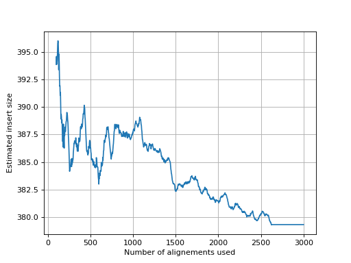
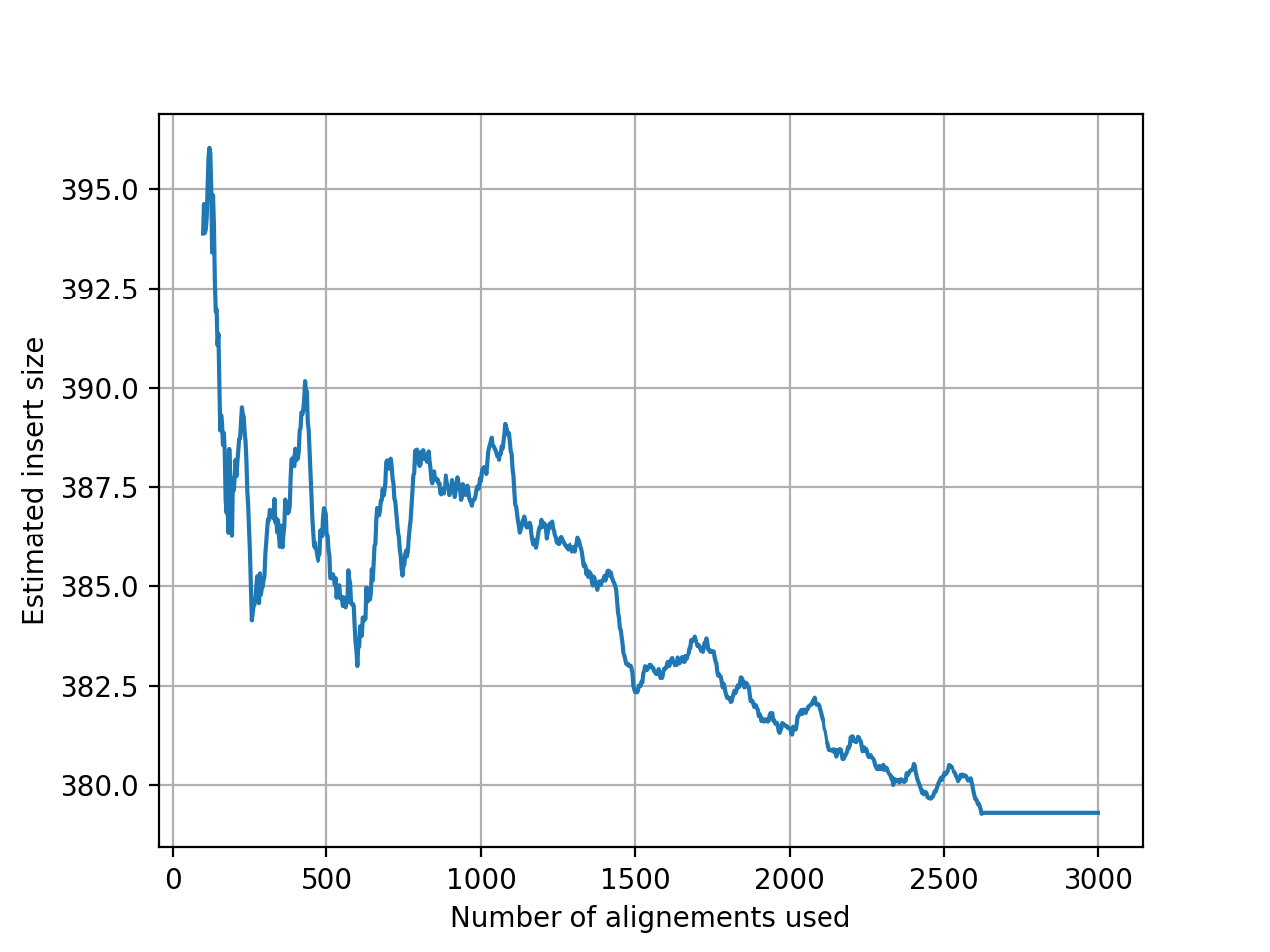
get_estimate_insert_size(max_entries=100000, upper_bound=1000, lower_bound=-1000)

Here we show that about 3000 alignments are enough to get a good estimate of the insert size.

(Source code, png, hires.png, pdf)

get_flags_as_df()

Returns decomposed flags as a dataframe

>>> from sequana import BAM, sequana_data
>>> b = BAM(sequana_data('test.bam'))
>>> df = b.get_flags_as_df()
>>> df.sum()
0          0
1       1000
2        484
4          2
8          2
16       499
32       500
64       477
128      523
256       64
512        0
1024       0
2048       0
dtype: int64

See also

SAMFlags for meaning of each flag

get_gc_content()

Return GC content for all reads (mapped or not)

See also

plot_gc_content()

get_length_count()

Return counter of all fragment lengths

get_mapped_read_length()

Return dataframe with read length for each read

(Source code, png, hires.png, pdf)

get_mapq_as_df(max_entries=-1)

Return dataframe with mapq for each read

get_query_end(read)

Get end of the query read.

get_query_start(read)

Get start of the query read.

get_read_names()

Return the reads' names

get_samflags_count()

Count how many reads have each flag of SAM format.

Returns:

dictionary with keys as SAM flags

get_samtools_stats_as_df()

Return a dictionary with full stats about the BAM/SAM file

The index of the dataframe contains the flags. The column contains the counts.

>>> from sequana import BAM, sequana_data
>>> b = BAM(sequana_data("test.bam"))
>>> df = b.get_samtools_stats_as_df()
>>> df.query("description=='average quality'")
36.9

Note

uses samtools behind the scene

get_stats()

Return basic stats about the reads

Returns:

dictionary with basic stats:

• total_reads : number reads ignoring supplementaty and secondary reads

• mapped_reads : number of mapped reads

• unmapped_reads : number of unmapped

• mapped_proper_pair : R1 and R2 mapped face to face

• reads_duplicated: number of reads duplicated

Warning

works only for BAM files. Use get_samtools_stats_as_df() for SAM files.

get_stats_full(mapq=30, max_entries=-1)

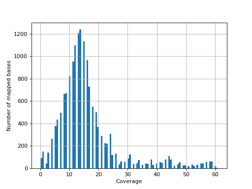
hist_coverage(chrom=None, bins=100)

from sequana import sequana_data, BAM
b = BAM(sequana_data("measles.fa.sorted.bam"))
b.hist_coverage()

(Source code, png, hires.png, pdf)

hist_soft_clipping()

histogram of soft clipping length ignoring supplementary and secondary reads

infer_strandness(reference_bed, max_entries, mapq=30)

Parameters:

• reference_bed -- a BED file (12-columns with columns 1,2,3,6 used) or GFF file (column 1, 3, 4, 5, 6 are used

• mapq -- ignore alignment with mapq below 30.

• max_entries -- can be long. max_entries restrict the estimate

Strandness of transcript is determined from annotation while strandness of reads is determined from alignments.

For non strand-specific RNA-seq data, strandness of reads and strandness of transcript are independent.

For strand-specific RNA-seq data, strandness of reads is determined by strandness of transcripts.

This functions returns a list of 4 values. First one indicates whether data is paired or not. Second and third one are ratio of reads explained by two types of strandness of reads vs transcripts. Last values are fractions of reads that could not be explained. The values 2 and 3 tell you whether this is a strand-specificit dataset.

If similar, it is no strand-specific. If the first value is close to 1 while the other is close to 0, this is a strand-specific dataset

property is_paired

property is_sorted

return True if the BAM is sorted

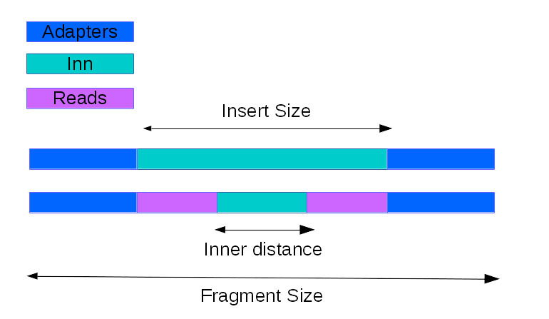
mRNA_inner_distance(refbed, low_bound=-250, up_bound=250, step=5, sample_size=1000000, q_cut=30)

Estimate the inner distance of mRNA pair end fragment.

from sequana import BAM, sequana_data
b = BAM(sequana_data("test_hg38_chr18.bam"))
df = b.mRNA_inner_distance(sequana_data("hg38_chr18.bed"))

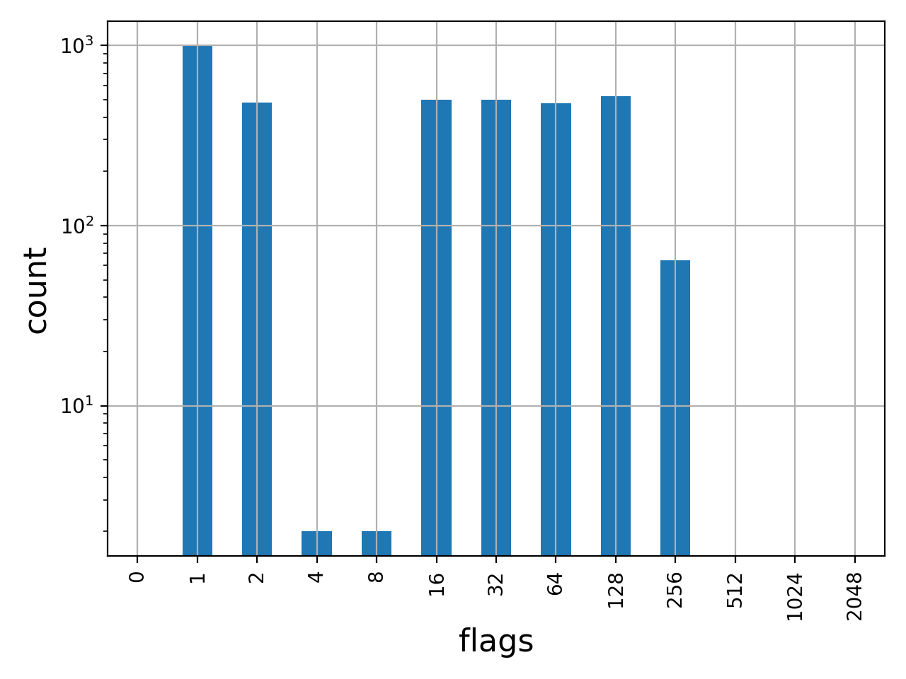
plot_bar_flags(logy=True, fontsize=16, filename=None)

Plot an histogram of the flags contained in the BAM

from sequana import BAM, sequana_data
b = BAM(sequana_data('test.bam'))
b.plot_bar_flags()

(Source code, png, hires.png, pdf)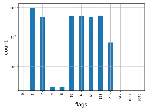

See also

SAMFlags for meaning of each flag

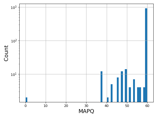
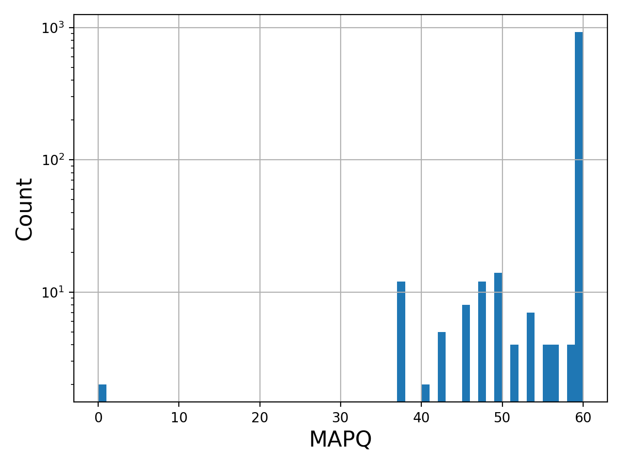
plot_bar_mapq(fontsize=16, filename=None)

Plots bar plots of the MAPQ (quality) of alignments

from sequana import BAM, sequana_data
b = BAM(sequana_data('test.bam'))
b.plot_bar_mapq()

(Source code, png, hires.png, pdf)

plot_coverage(chrom=None)

Please use SequanaCoverage for more sophisticated tools to plot the genome coverage

from sequana import sequana_data, BAM
b = BAM(sequana_data("measles.fa.sorted.bam"))
b.plot_coverage()

(Source code, png, hires.png, pdf)

plot_gc_content(fontsize=16, ec='k', bins=100)

plot GC content histogram

Params bins:

a value for the number of bins or an array (with a copy() method)

Parameters:

ec -- add black contour on the bars

from sequana import BAM, sequana_data
b = BAM(sequana_data('test.bam'))
b.plot_gc_content()

(Source code, png, hires.png, pdf)

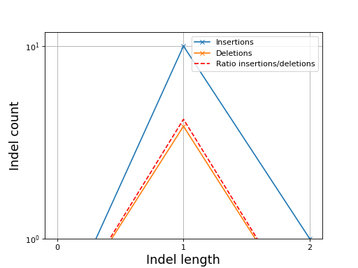
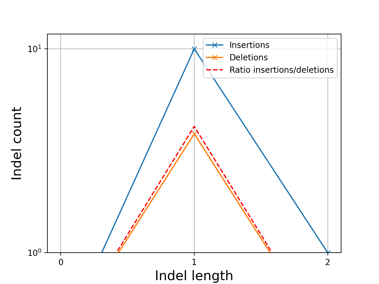
plot_indel_dist(fontsize=16)

Plot indel count (+ ratio)

Return:

list of insertions, deletions and ratio insertion/deletion for different length starting at 1

from sequana import sequana_data, BAM
b = BAM(sequana_data("measles.fa.sorted.bam"))
b.plot_indel_dist()

(Source code, png, hires.png, pdf)

What you see on this figure is the presence of 10 insertions of length 1, 1 insertion of length 2 and 3 deletions of length 1

# Note that in samtools, several insertions or deletions in a single alignment are ignored and only the first one seems to be reported. For instance 10M1I10M1I stored only 1 insertion in its report; Same comment for deletions.

Todo

speed up and handle long reads cases more effitiently by storing INDELS as histograms rather than lists

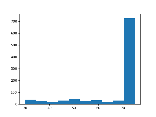
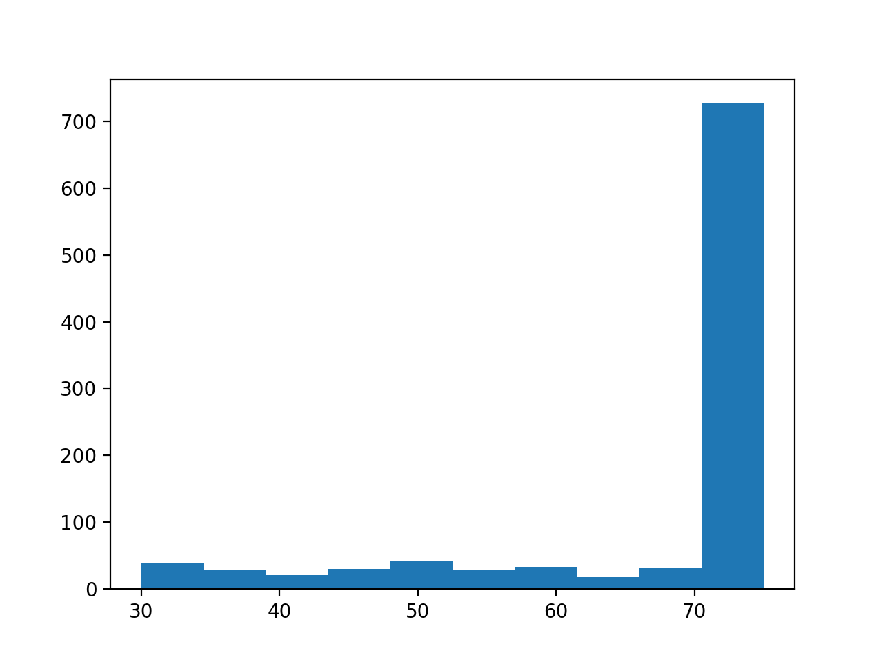
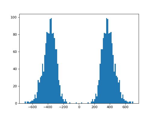
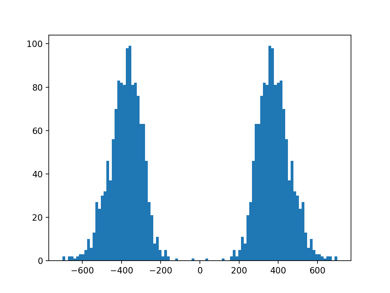
plot_insert_size(max_entries=100000, bins=100, upper_bound=1000, lower_bound=-1000, absolute=False)

This gives an idea of the insert size without taking into account any intronic gap. The mode should give a good idea of the insert size though.

(Source code, png, hires.png, pdf)

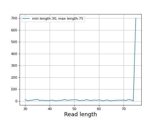
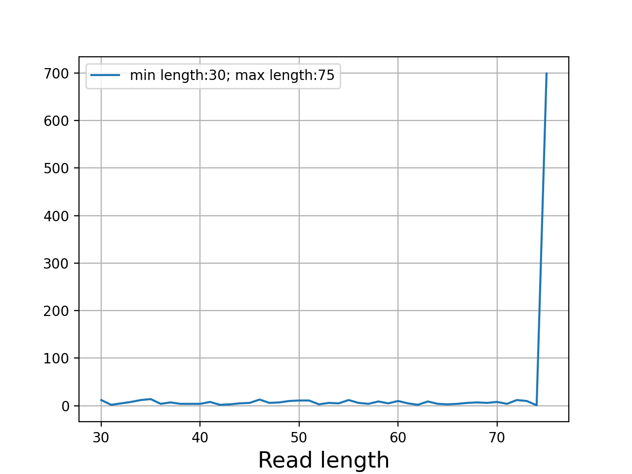
plot_read_length()

Plot occurences of aligned read lengths

from sequana import sequana_data, BAM
b = BAM(sequana_data("test.bam"))
b.plot_read_length()

(Source code, png, hires.png, pdf)

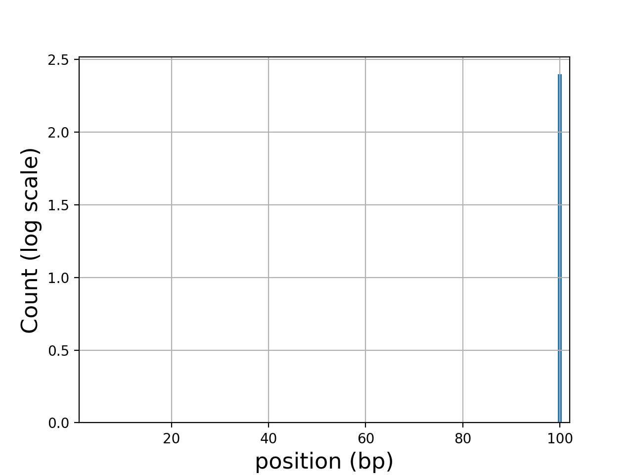
plotly_hist_read_length(log_y=False, title='', xlabel='Read length (bp)', ylabel='count', **kwargs)

Histogram of the read length using plotly

Parameters:

• log_y --

• title --

any additional arguments is pass to the plotly.express.hist function

reset()

property summary

Count flags/mapq/read length in one pass.

to_fastq(filename)

Export the BAM to FastQ format

Todo

comments from original reads are not in the BAM so will be missing

Method 1 (bedtools):

bedtools bamtofastq -i JB409847.bam  -fq test1.fastq

Method2 (samtools):

samtools bam2fq JB409847.bam > test2.fastq

Method3 (sequana):

from sequana import BAM
BAM(filename)
BAM.to_fastq("test3.fastq")

Note that the samtools method removes duplicated reads so the output is not identical to method 1 or 3.

to_paf()

class SAMFlags(value=4095)

Utility to extract bits from a SAM flag

>>> from sequana import SAMFlags
>>> sf = SAMFlags(257)
>>> sf.get_flags()
[1, 256]

You can also print the bits and their description:

print(sf)

bit	Meaning/description
0	mapped segment
1	template having multiple segments in sequencing
2	each segment properly aligned according to the aligner
4	segment unmapped
8	next segment in the template unmapped
16	SEQ being reverse complemented
32	SEQ of the next segment in the template being reverse complemented
64	the first segment in the template
128	the last segment in the template
256	secondary alignment
512	not passing filters, such as platform/vendor quality controls
1024	PCR or optical duplicate
2048	supplementary alignment

Reference:

http://samtools.github.io/hts-specs/SAMv1.pdf

get_flags()

Return the individual bits included in the flag

get_meaning()

Return all description sorted by bit

11.3. Coverage (bedtools module)

Utilities for the genome coverage

class ChromosomeCov(genomecov, chrom_name, thresholds=None, chunksize=5000000)

Factory to manipulate coverage and extract region of interests.

Example:

from sequana import SequanaCoverage, sequana_data
filename = sequana_data("virus.bed")

gencov = SequanaCoverage(filename)

chrcov = gencov[0]
chrcov.running_median(n=3001)
chrcov.compute_zscore()
chrcov.plot_coverage()

df = chrcov.get_rois().get_high_rois()

(Source code, png, hires.png, pdf)

The df variable contains a dataframe with high region of interests (over covered)

If the data is large, the input data set is split into chunk. See chunksize, which is 5,000,000 by default.

If your data is larger, then you should use the run() method.

See also

sequana_coverage standalone application

constructor

Parameters:

• df -- dataframe with position for a chromosome used within SequanaCoverage. Must contain the following columns: ["pos", "cov"]

• genomecov --

• chrom_name -- to save space, no need to store the chrom name in the dataframe.

• thresholds -- a data structure DoubleThresholds that holds the double threshold values.

• chunksize -- if the data is large, it is split and analysed by chunk. In such situations, you should use the run() instead of calling the running_median and compute_zscore functions.

property BOC

breadth of coverage

property C3

property C4

property CV

The coefficient of variation (CV) is defined as sigma / mu

property DOC

depth of coverage

property STD

standard deviation of depth of coverage

property bed

compute_zscore(k=2, use_em=True, clip=4, verbose=True)

Compute zscore of coverage and normalized coverage.

Parameters:

• k (int) -- Number gaussian predicted in mixture (default = 2)

• clip (float) -- ignore values above the clip threshold

Store the results in the df attribute (dataframe) with a column named zscore.

Note

needs to call running_median() before hand.

property df

property evenness

Return Evenness of the coverage

Reference:

Konrad Oexle, Journal of Human Genetics 2016, Evaulation of the evenness score in NGS.

work before or after normalisation but lead to different results.

get_centralness(threshold=3)

Proportion of central (normal) genome coverage

This is 1 - (number of non normal data) / (total length)

Note

depends on the thresholds attribute being used.

Note

depends slightly on the running median window

get_gaussians()

get_gc_correlation()

Return the correlation between the coverage and GC content

The GC content is the one computed in SequanaCoverage.compute_gc_content() (default window size is 101)

get_rois()

Keep positions with zscore outside of the thresholds range.

Returns:

a dataframe from FilteredGenomeCov

Note

depends on the thresholds low and high values.

get_stats()

Return basic stats about the coverage data

only "cov" column is required.

Returns:

dictionary

get_summary(C3=None, C4=None, stats=None, caller='sequana.bedtools')

init()

moving_average(n, circular=False)

Compute moving average of the genome coverage

Parameters:

• n -- window's size. Must be odd

• circular (bool) -- is the chromosome circular or not

Store the results in the df attribute (dataframe) with a column named ma.

next()

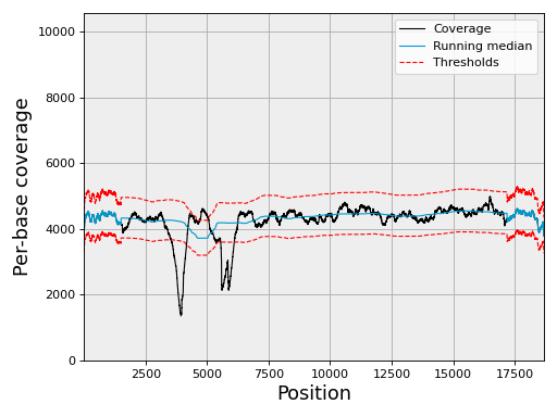
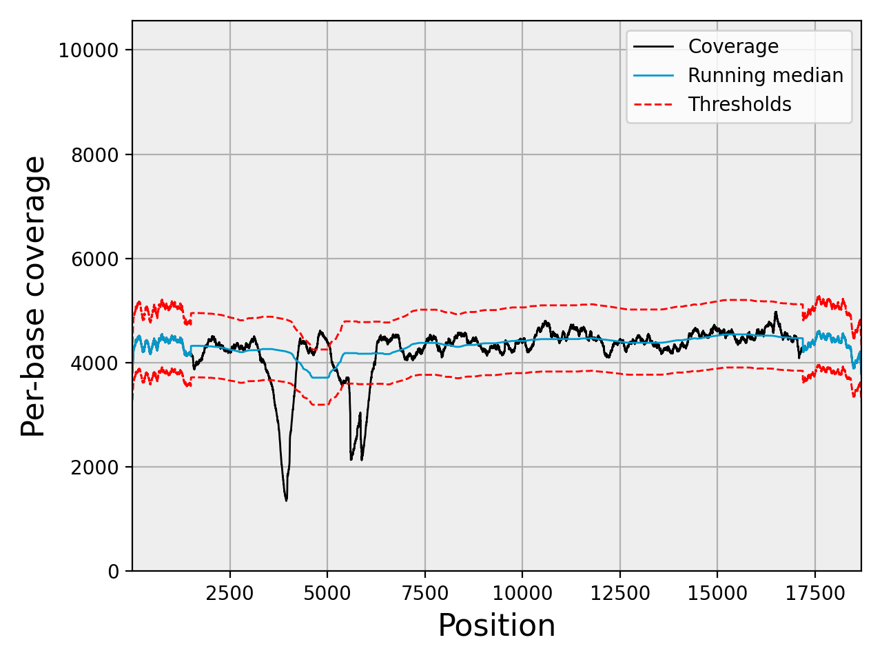
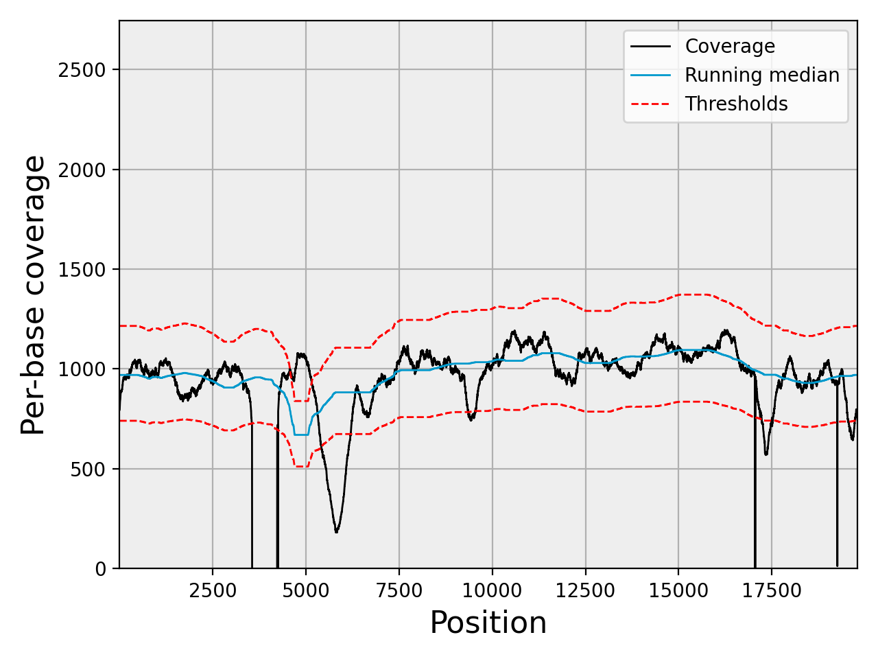
plot_coverage(filename=None, fontsize=16, rm_lw=1, rm_color='#0099cc', rm_label='Running median', th_lw=1, th_color='r', th_ls='--', main_color='k', main_lw=1, main_kwargs={}, sample=True, set_ylimits=True, x1=None, x2=None, clf=True)

Plot coverage as a function of base position.

Parameters:

• filename --

• rm_lw -- line width of the running median

• rm_color -- line color of the running median

• rm_color -- label for the running median

• th_lw -- line width of the thresholds

• th_color -- line color of the thresholds

• main_color -- line color of the coverage

• main_lw -- line width of the coverage

• sample -- if there are more than 1 000 000 points, we use an integer step to skip data points. We can still plot all points at your own risk by setting this option to False

• set_ylimits -- we want to focus on the "normal" coverage ignoring unsual excess. To do so, we set the yaxis range between 0 and a maximum value. This maximum value is set to the minimum between the 10 times the mean coverage and 1.5 the maximum of the high coverage threshold curve. If you want to let the ylimits free, set this argument to False

• x1 -- restrict lower x value to x1

• x2 -- restrict lower x value to x2 (x2 must be greater than x1)

Note

if there are more than 1,000,000 points, we show only 1,000,000 by points. For instance for 5,000,000 points,

In addition to the coverage, the running median and coverage confidence corresponding to the lower and upper zscore thresholds are shown.

Note

uses the thresholds attribute.

plot_gc_vs_coverage(filename=None, bins=None, Nlevels=None, fontsize=20, norm='log', ymin=0, ymax=100, contour=True, cmap='BrBG', **kwargs)

Plot histogram 2D of the GC content versus coverage

plot_hist_coverage(logx=True, logy=True, fontsize=16, N=25, fignum=1, hold=False, alpha=0.8, ec='k', filename=None, zorder=10, **kw_hist)

Parameters:

• N --

• ec --

plot_hist_normalized_coverage(filename=None, binwidth=0.05, max_z=3)

Barplot of the normalized coverage with gaussian fitting

plot_hist_zscore(fontsize=16, filename=None, max_z=6, binwidth=0.5, **hist_kargs)

Barplot of the zscore values

plot_rois(x1, x2, set_ylimits=False, rois=None, fontsize=16, color_high='r', color_low='g', clf=True)

property rois

run(W, k=2, circular=False, binning=None, cnv_delta=None)

running_median(n, circular=False)

Compute running median of genome coverage

Parameters:

• n (int) -- window's size.

• circular (bool) -- if a mapping is circular (e.g. bacteria whole genome sequencing), set to True

Store the results in the df attribute (dataframe) with a column named rm.

Changed in version 0.1.21: Use Pandas rolling function to speed up computation.

to_csv(filename=None, start=None, stop=None, **kwargs)

Write CSV file of the dataframe.

Parameters:

• filename (str) -- csv output filename. If None, return string.

• start (int) -- start row index.

• stop (int) -- stop row index.

Params of pandas.DataFrame.to_csv():

Parameters:

• columns (list) -- columns you want to write.

• header (bool) -- determine if the header is written.

• index (bool) -- determine if the index is written.

• float_format (str) -- determine the float format.

class DoubleThresholds(low=-3, high=3, ldtr=0.5, hdtr=0.5)

Simple structure to handle the double threshold for negative and positive sides

Used by the SequanaCoverage and related classes.

dt = DoubleThresholds(-3, 4, 0.5, 0.5)

This means the low threshold is -3 while the high threshold is 4. The two following values must be between 0 and 1 and are used to define the value of the double threshold set to half the value of the main threshold.

Internally, the main thresholds are stored in the low and high attributes. The secondary thresholds are derived from the main thresholds and the two ratios. The ratios are named ldtr and hdtr for low double threshold ratio and high double threshold ratio. The secondary thresholds are denoted low2 and high2 and are update automatically if low, high, ldtr or hdtr are changed.

copy()

get_args()

property hdtr

property high

property high2

property ldtr

property low

property low2

class SequanaCoverage(input_filename, annotation_file=None, low_threshold=-4, high_threshold=4, ldtr=0.5, hdtr=0.5, force=False, chunksize=5000000, quiet_progress=False, chromosome_list=[], reference_file=None, gc_window_size=101)

Create a list of dataframe to hold data from a BED file generated with samtools depth.

This class can be used to plot the coverage resulting from a mapping, which is stored in BED format. The BED file may contain several chromosomes. There are handled independently and accessible as a list of ChromosomeCov instances.

Example:

from sequana import SequanaCoverage, sequana_data

filename = sequana_data('JB409847.bed')
reference = sequana_data("JB409847.fasta")

gencov = SequanaCoverage(filename)

# you can change the thresholds:
gencov.thresholds.low = -4
gencov.thresholds.high = 4
#gencov.compute_gc_content(reference)

gencov = SequanaCoverage(filename)
for chrom in gencov:
    chrom.running_median(n=3001, circular=True)
    chrom.compute_zscore()
    chrom.plot_coverage()
gencov[0].plot_coverage()

(Source code)

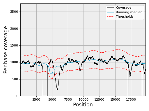
Results are stored in a list of ChromosomeCov named chr_list. For Prokaryotes and small genomes, this API is convenient but takes lots of memory for larger genomes.

Computational time information: scanning 24,000,000 rows

• constructor (scanning 40,000,000 rows): 45s

• select contig of 24,000,000 rows: 1min20

• running median: 16s

• compute zscore: 9s

• c.get_rois() ():

constructor

Parameters:

• input_filename (str) -- the input data with results of a bedtools genomecov run. This is just a 3-column file. The first column is a string (chromosome), second column is the base postion and third is the coverage.

• annotation_file (str) -- annotation file of your reference (GFF3/Genbank).

• low_threshold (float) -- threshold used to identify under-covered genomic region of interest (ROI). Must be negative

• high_threshold (float) -- threshold used to identify over-covered genomic region of interest (ROI). Must be positive

• ldtr (float) -- fraction of the low_threshold to be used to define the intermediate threshold in the double threshold method. Must be between 0 and 1.

• rdtr (float) -- fraction of the low_threshold to be used to define the intermediate threshold in the double threshold method. Must be between 0 and 1.

• chunksize -- size of segments to analyse. If a chromosome is larger than the chunk size, it is split into N chunks. The segments are analysed indepdently and ROIs and summary joined together. Note that GC, plotting functionalities will only plot the first chunk.

• force -- some constraints are set in the code to prevent unwanted memory issues with specific data sets of parameters. Currently, by default, (i) you cannot set the threshold below 2.5 (considered as noise).

• chromosome_list -- list of chromosomes to consider (names). This is useful for very large input data files (hundreds million of lines) where each chromosome can be analysed one by one. Used by the sequana_coverage standalone. The only advantage is to speed up the constructor creation and could also be used by the Snakemake implementation.

• reference_file -- if provided, computes the GC content

• gc_window_size (int) -- size of the GC sliding window. (default 101)

property annotation_file

Get or set the genbank filename to annotate ROI detected with ChromosomeCov.get_roi(). Changing the genbank filename will configure the SequanaCoverage.feature_dict.

property circular

Get the circularity of chromosome(s). It must be a boolean.

property feature_dict

Get the features dictionary of the genbank.

property gc_window_size

Get or set the window size to compute the GC content.

get_stats()

Return basic statistics for each chromosome

Returns:

dictionary with chromosome names as keys and statistics as values.

See also

ChromosomeCov.

Note

used in sequana_summary standalone

property input_filename

property reference_file

property window_size

Get or set the window size to compute the running median. Size must be an interger.

11.4. CIGAR tools

class Cigar(cigarstring)

>>> from sequana.cigar import Cigar
>>> c = Cigar("2S30M1I")
>>> len(c)
33

>>> c = Cigar("1S1S1S1S")
>>> c.compress()
>>> c.cigarstring
'4S'

Possible CIGAR types are:

• "M" for alignment MATCH (0)

• "I" for Insertion to the reference (1)

• "D" for deletion from the reference 2

• "N" for skipped region from the reference 3

• "S" for soft clipping (clipped sequence present in seq) 4

• "H" for hard clipping (clipped sequence NOT present in seq) 5

• "P" for padding (silent deletion from padded reference)

• "=" for equal

• "X" for diff (sequence mismatched)

• "B" for back !!!! could be also NM ???

!!! BWA MEM get_cigar_stats returns list with 11 items Last item is !!! what is the difference between M and = ??? Last item is I + S + X !!! dans BWA, mismatch (X) not provided... should be deduced from last item - I - S

Note

the length of the query sequence based on the CIGAR is calculated by adding the M, I, S, =, or X and other operations are ignored. source: https://stackoverflow.com/questions/39710796/infer-the-length-of-a-sequence-using-the-cigar/39812985#39812985

Reference:

https://github.com/samtools/htslib/blob/develop/htslib/sam.h

Constructor

Parameters:

cigarstring (str) -- the CIGAR string.

Note

the input CIGAR string validity is not checked. If an unknown type is found, it is ignored generally. For instance, the length of 1S100Y is 1 since Y is not correct.

as_dict()

Return cigar types and their count

Returns:

dictionary

Note that repeated types are added:

>>> c = Cigar('1S2M1S')
>>> c.as_dict()
{"S":2,"M":2}

as_sequence()

as_tuple()

Decompose the cigar string into tuples keeping track of repeated types

Returns:

tuple

>>> from sequana import Cigar
>>> c = Cigar("1S2M1S")
>>> c.as_tuple()
(('S', 1), ('M', 2), ('S', 1))

cigarstring

the CIGAR string attribute

compress()

1S1S should become 2S. inplace modification

pattern = '(\\d+)([A-Za-z])?'

stats()

Returns number of occurence for each type found in types

>>> c = Cigar("1S2M1S")
>>> c.stats()
[2, 0, 0, 0, 2, 0, 0, 0, 0, 0]

types = 'MIDNSHP=XB'

valid CIGAR types

fetch_clip(chrom, start, cigar)

fetch_deletion(chrom, start, cigar)

fetch_exon(chrom, start, cigar)

fetch_insertion(chrom, start, cigar)

fetch_intron(chrom, start, cigar)

11.5. Coverage (theoretical)

class Coverage(N=None, L=None, G=None, a=None)

Utilities related to Lander and Waterman theory

We denote the genome length in nucleotides and the read length in nucleotides. These two numbers are in principle well defined since is defined by biology and by the sequencing machine.

The total number of reads sequenced during an experiment is denoted . Therefore the total number of nucleotides is simply .

The depth of coverage (DOC) at a given nucleotide position is the number of times that a nucleotide is covered by a mapped read.

The theoretical fold-coverage is defined as :

that is the average number of times each nucleotide is expected to be sequenced (in the whole genome). The fold-coverage is often denoted (e.g., 50X).

In the Coverage class, and are fixed at the beginning. Then, if one changes , then is updated and vice-versa so that the relation is always true:

>>> cover = Coverage(G=1000000, L=100)
>>> cover.N = 100000    # number of reads
>>> cover.a             # What is the mean coverage
10
>>> cover.a = 50
>>> cover.N
500000

From the equation aforementionned, and assuming the reads are uniformly distributed, we can answer a few interesting questions using probabilities.

In each chromosome, a read of length could start at any position (except the last position L-1). So in a genome with chromosomes, there are possible starting positions. In general so the probability that one of the read starts at any specific nucleotide is .

The probability that a read (of length ) covers a given position is . The probability of not covering that location is . For fragments, we obtain the probability . So, the probability of covering a given location with at least one read is :

Since in general, N>>1, we have:

From this equation, we can derive the fold-coverage required to have e.g., of the genome covered:

equivalent to

The method get_required_coverage() uses this equation. However, for numerical reason, one should not provide as an argument but (1-E). See get_required_coverage()

Other information can also be derived using the methods get_mean_number_contigs(), get_mean_contig_length(), get_mean_contig_length().

See also

get_table() that provides a summary of all these quantities for a range of coverage.

Reference:

http://www.math.ucsd.edu/~gptesler/283/FA14/slides/shotgun_14-handout.pdf

property G

genome length

property L

length of the reads

property N

number of reads defined as aG/L

property a

coverage defined as NL/G

get_mean_contig_length()

Expected length of the contigs

get_mean_number_contigs()

Expected number of contigs

A binomial distribution with parameters and

get_mean_reads_per_contig()

Expected number of reads per contig

Number of reads divided by expected number of contigs:

get_percent_genome_sequenced()

Return percent of the genome covered

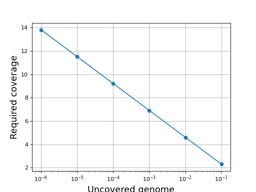
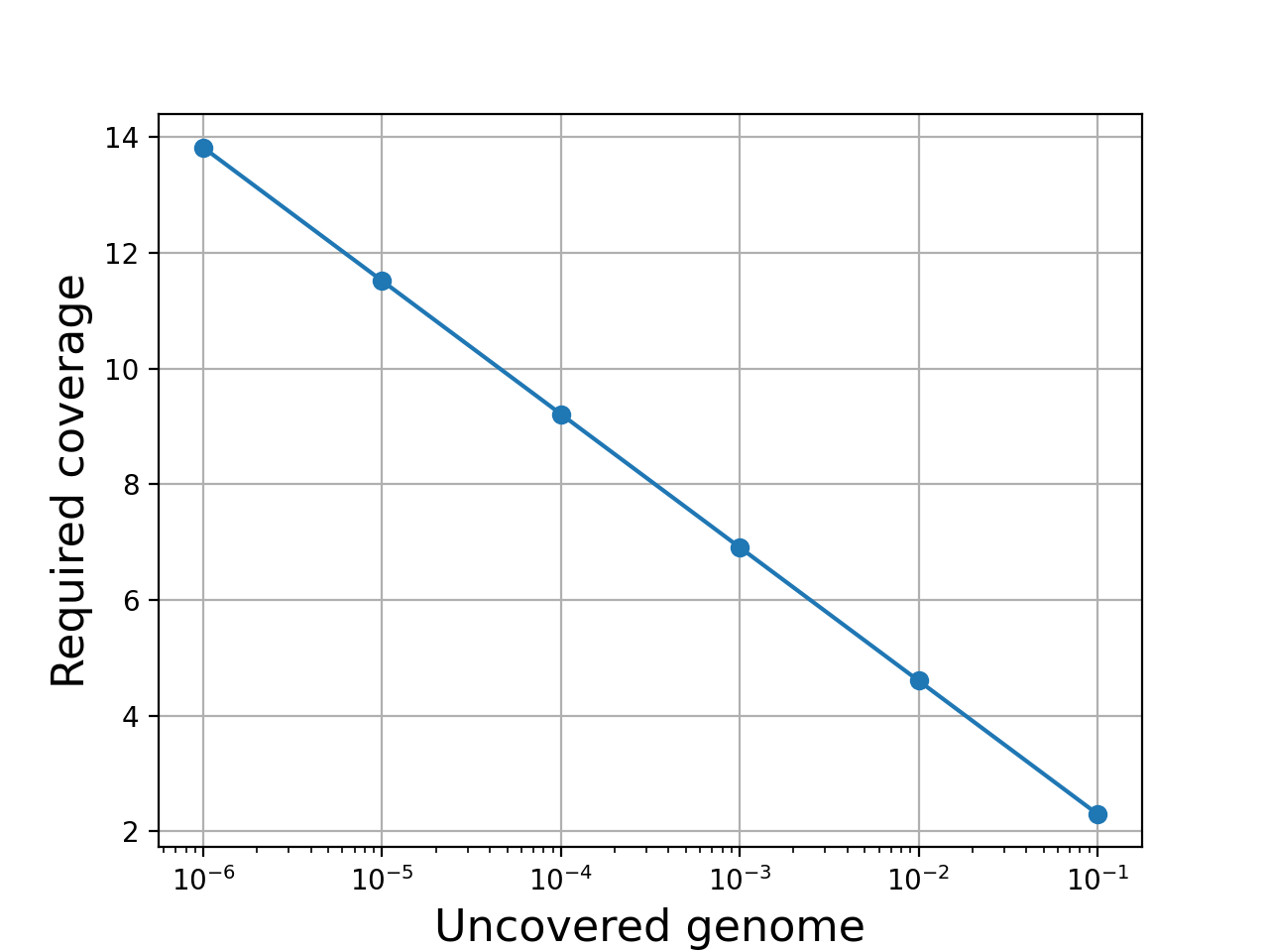
get_required_coverage(M=0.01)

Return the required coverage to ensure the genome is covered

A general question is what should be the coverage to make sure that e.g. E=99% of the genome is covered by at least a read.

The answer is:

This equation is correct but have a limitation due to floating precision. If one provides E=0.99, the answer is 4.6 but we are limited to a maximum coverage of about 36 when one provides E=0.9999999999999999 after which E is rounded to 1 on most computers. Besides, it is no convenient to enter all those numbers. A scientific notation would be better but requires to work with instead of .

So instead of asking the question what is the requested fold coverage to have 99% of the genome covered, we ask the question what is the requested fold coverage to have 1% of the genome not covered. This allows us to use values as low as 1e-300 that is a fold coverage as high as 690.

Parameters:

M (float) -- this is the fraction of the genome not covered by any reads (e.g. 0.01 for 1%). See note above.

Returns:

the required fold coverage

(Source code, png, hires.png, pdf)

# The inverse equation is required fold coverage = [log(-1/(E - 1))]

get_summary()

Return a summary (dictionary) for the current fold coverage a

get_table(coverage=None)

Return a summary dataframe for a set of fold coverage

Parameters:

coverage (list) -- if None, coverage list starts at 0.5 and ends at 10 with a step of 0.5

11.6. Access to online database (e.g. ENA)

Utilities to access to online FASTA, taxon, lineage ...

class ENADownload

Downloader to retrieve genome fasta files from ENA amongst other things

In order to facilitate the download of FASTA files (e.g. to build a Kraken DB), this class can be used to download a bunch of FASTA files, or just one given its accession.

Some OLD pre-defined lists are available from ENA. We refer to them as virus, plasmid, phage, archaealvirus, archaea, bacteria, organelle, viroid.

Warning

the header of the FASTA files are changed to add the GI number instead of embl so th&at it can be used by our kraken builder class.

constructor

add_gi_to_header(acc)

Kraken will only accept the GI from NCBI so we need to convert the ENA accession to GI numbers

download_fasta(filelist, output_dir=None)

Download a FASTA (or list of)

Parameters:

filelist -- a name to find on the ENA web server OR the name of an accession number or a file with accession numbers (1 column)

Warning

The filename is named after the accession without .X number If there are several variant .1, .2 the later will be used. This should not happen if the list is properly defined.

ena_id_to_gi_number(identifiers)

class EUtilsTools

Utilities to fetch information about accession numbers

>>> from sequana.databases import EUtilsTools
>>> et = EUtilsTools()
>>> et.accession_to_info("K01711.1")
{'K01711.1': {'accession': '331784',
  'comment': 'Measles virus (strain Edmonston), complete genome',
  'gi': '331784',
  'identifier': 'gi|331784|gb|K01711.1|MEANPCG[331784]',
  'taxid': '11234'}}

accession_to_info(ids)

An accession or list of them returns list of dictionaries

get_fasta(accession)

class NCBIDownload

download_assembly_report(category, output=None)

download_genomes_from_ncbi(category, email='sequana@pasteur.fr')

This downloads all genomes on ncbi for a given category looking at their ftp. This could be highly redundant.

download_ncbi_refseq_release(category, email='sequana@pasteur.fr', outdir='.')

Download all files of type fna from ncbi FTP.

kb = NCBIDownload()
kb.download_ncbi_refseq_release("viral")

class NCBITaxonReader(names=None, nodes=None)

This class will help in reading, handling, simplifying NCBI taxonomic DB

When downloading NCBI taxonomy DB using e.g. Kraken, we end up with very large files. One is called names.dmp and the other nodes.dmp. They may be instrospected or simplified using this class

The names.dmp is just a CSV file. The header looks like:

1   |   all |       |   synonym |
1   |   root    |       |   scientific name |
2   |   Bacteria    |   Bacteria <prokaryote>   |   scientific name |
2   |   Monera  |   Monera <Bacteria>   |   in-part |
2   |   Procaryotae |   Procaryotae <Bacteria>  |   in-part |

It is a tabulated file. If we ignore the | signs, it contains 4 columns:

taxid
name
unique name
type of name

The unique name column is generally empty and is dropped internally. There are different types of name, so there can be several rows for a given taxid. For instance for the taxon 1, there isa scientific name and a synonym

The df_name is a dataframe that stores the taxid, name and type of name in a dataframe.

The second file 'nodes.dmp') looks like:

1 | 1       | no rank |     | 8 | 0 | 1  | 0  | 0 | 0 | 0 | 0 |   |
2 | 131567  | superkingdom  |   | 0 | 0  | 11 | 0 | 0 | 0 | 0 | 0 | |
6 | 335928  | genus   |     | 0 | 1 | 11 | 1  | 0 | 1 | 0 | 0 |   |
7 | 6       | species | AC  | 0 | 1 | 11 | 1  | 0 | 1 | 1 | 0 |   |
9 | 32199   | species | BA  | 0 | 1 | 11 | 1  | 0 | 1 | 1 | 0 |   |

Again this is a tabulated file. The first three columns are taxid, parent taxid, and rank. Rank is species, genus, family, phylum, etc. Newest version of nodes.dmp hqs only 4 columns (taxid, parent taxid, rank ,a dash)

from sequana.databases import NCBITaxonReader

# The first time you may want to download the taxdump files
n = NCBITaxonReader()
n.download_taxdump()
n.init("names.dmp", "nodes.dmp")

# next time, you can read it directly
n.NCBITaxonReader("names.dmp", "nodes.dmp")

Constructor

Parameters:

• names (str) -- Defaults to "names.dmp".

• nodes (str) -- Defaults to "nodes.dmp".

download_taxdump(outpath='.')

filter_names_dmp_file(output='names_filtered.dmp', taxons=[])

Save a subset of nodes.dmp given list of valid taxons

Parameters:

• str -- Defaults to "nodes_filtered.dmp".

• taxons (list) --

filter_nodes_dmp_file(output='nodes_filtered.dmp', taxons=[])

Save a subset of nodes.dmp given list of valid taxons

Parameters:

• str -- Defaults to "nodes_filtered.dmp".

• taxons (list) --

ftp_url = 'ftp.ncbi.nih.gov'

get_average_name_per_taxon()

Return number of rows/names per node/taxon

get_family(taxon)

Get all parent taxons

get_number_taxon()

Return number of unique taxon

get_scientific_name(taxon)

Return scientific name of a given Taxon

get_taxon_from_scientific_name(scname)

Return taxon corresponding to a scientific name

return: unique taxon or first one found. If none found, returns None

init(names, nodes)

search(name)

Search names colum

11.7. Enrichment

11.8. Experimental design

IEM class

class IEM(filename)

Reader and validator of IEM samplesheets

The IEM samplesheet reader and validator verifies the correctness of the sections in the samplesheet, which are case-sensitive and are enclosed within square brackets. Following the closing bracket, no additional characters are permitted, except for commas and the end-of-line marker.

The samplesheet must start with the [Header] section and end with the [Data] section, with other sections arranged arbitrarily.

The [Header] section must appear on the first line and consist of key-value pairs represented as records, with each line consisting of precisely two fields.

An optional [Settings] section can contain key-value pairs, and the [Reads] section specifies the number of cycles per read, which is exclusively required for MiSeq.

For the IEM samplesheet with adapters, the following fields must be present: [Version], [Name], [Settings], [I7], [I5], [IndexPlateLayout].

The [Data] section, which is a table similar to CSV format, is required and must be located at the end of the samplesheet file. There are no specific ordering requirements for column names, and they are not case-sensitive. At the very least, each sample must have a unique string identifier in the Sample_ID column.

Example of typical Data section to be used with bcl2fastq:

[Header]

[Data]
Sample_ID,Sample_Name,I7_Index_ID,index,I5_INdex_ID,index2
A10001,Sample_A,D701,AATACTCG,D501,TATAGCCT
A10002,Sample_B,D702,TCCGGAGA,D501,TATAGCCT
A10003,Sample_C,D703,CGCTCATT,D501,TATAGCCT
A10004,Sample_D,D704,GAGATTCC,D501,TATAGCCT

Sequana Standalone

The standalone application sequana contains a subcommand based on this class:

sequana samplesheet

that can be used to check the correctness of a samplesheet:

sequana samplesheet --check SampleSheet.csv

References:

illumina specifications 970-2017-004.pdf

checker()

property df

Returns the [data] section

expected_data_headers = {'PE': [], 'SE': []}

expected_headers_fields = ['IEMFileVersion', 'Investigator Name', 'Instrument Type', 'Experiment Name', 'Date', 'Workflow', 'Application', 'Assay', 'Description', 'Chemistry', 'Index Adapters']

expected_settings_fields = ['Adapter', 'ReverseComplement', 'CustomRead1PrimerMix']

property header

property index_adapters

returns index adapters

property instrument

returns instrument name

property name

quick_fix(output_filename)

Fix sample sheet

Tyical error is when users save the samplesheet as CSV file in excel. This may add trailing ; characters at the end of section, which raises error in bcl2fastq.

property samples

returns the sample identifiers as a list

property settings

to_fasta(adapter_name='')

Extract adapters from [Adapter] section and print them as a fasta file

validate()

This method checks whether the sample sheet is correctly formatted

Checks for:

• presence of ; at the end of lines indicated an edition with excel that wrongly transformed the data into a pure CSV file

• inconsistent numbers of columns in the [DATA] section, which must be CSV-like section

• Extra lines at the end are ignored

• special characters are forbidden except - and _

• checks for Sample_ID column uniqueness

• checks for index uniqueness (if single index)

• checks for combo of dual indices uniqueness

• checks that sample names are unique

and raise a SystemExit error on the first found error.

property version

return the version of the IEM file

11.9. FASTQ module

Utilities to manipulate FASTQ and Reads

class FastQ(filename, verbose=False)

Class to handle FastQ files

Some of the methods are based on pysam but a few are also original to sequana. In general, input can be zipped ot not and output can be zipped or not (based on the extension).

An example is the extract_head() method:

f = FastQ("input_file.fastq.gz")
f.extract_head(100000, output='test.fastq')
f.extract_head(100000, output='test.fastq.gz')

equivalent to:

zcat myreads.fastq.gz | head -100000 | gzip > test100k.fastq.gz

An efficient implementation to count the number of lines is also available:

f.count_lines()

or reads (assuming 4 lines per read):

f.count_reads()

Operators available:

• equality ==

count_lines()

Return number of lines

count_reads()

Return count_lines divided by 4

extract_head(N, output_filename)

Extract the heads of a FastQ files

Parameters:

• N (int) --

• output_filename (str) -- Based on the extension the output file is zipped or not (.gz extension only)

This function is convenient since it takes into account the input file being compressed or not and the output file being compressed ot not. It is in general 2-3 times faster than the equivalent unix commands combined together but is 10 times slower for the case on uncompressed input and uncompressed output.

Warning

this function extract the N first lines and does not check if there are empty lines in your FastQ/FastA files.

filter(identifiers_list=[], min_bp=None, max_bp=None, progress=True, output_filename='filtered.fastq')

Save reads in a new file if there are not in the identifier_list

Parameters:

• min_bp (int) -- ignore reads with length shorter than min_bp

• max_bp (int) -- ignore reads with length above max_bp

get_lengths()

joining(pattern, output_filename)

not implemented

zcat Block*.fastq.gz | gzip > combined.fastq.gz

property n_lines

return number of lines (should be 4 times number of reads)

property n_reads

return number of reads

next()

rewind()

Allows to iter from the beginning without openning the file or creating a new instance.

select_random_reads(N=None, output_filename='random.fastq', progress=True)

Select random reads and save in a file

Parameters:

• N (int) -- number of random unique reads to select should provide a number but a list can be used as well. You can select random reads for R1, and re-use the returned list as input for the R2 (since pairs must be kept)

• output_filename (str) --

If you have a pair of files, the same reads must be selected in R1 and R2.:

f1 = FastQ(file1)
selection = f1.select_random_reads(N=1000)
f2 = FastQ(file2)
f2.select_random_reads(selection)

Changed in version 0.9.8: use list instead of set to keep integrity of paired-data

select_reads(read_identifiers, output_filename=None, progress=True)

identifiers must be the name of the read without starting @ sign and without comments.

split_chunks(N=10)

Not implemented

split_lines(N=100000, gzip=True)

Not implemented

stats()

to_fasta(output_filename='test.fasta')

Slow but works for now in pure python with input compressed data.

to_kmer_content(k=7)

Return a Series with kmer count across all reads

Parameters:

k (int) -- (default to 7-mers)

Returns:

Pandas Series with index as kmer and values as count.

Takes about 30 seconds on a million reads.

to_krona(k=7, output_filename='fastq.krona')

Save Krona file with ACGT content within all k-mers

Parameters:

k (int) -- (default to 7-mers)

Save results in file, which can then be translated into a HTML file using:

ktImportText fastq.krona
open text.krona.html

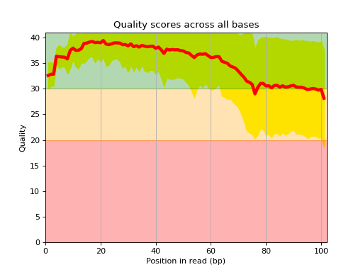
class FastQC(filename, max_sample=500000, verbose=True, skip_nrows=0)

Simple QC diagnostic

Similarly to some of the plots of FastQC tools, we scan the FastQ and generates some diagnostic plots. The interest is that we'll be able to create more advanced plots later on.

Here is an example of the boxplot quality across all bases:

from sequana import sequana_data
from sequana import FastQC
filename  = sequana_data("test.fastq", "doc")
qc = FastQC(filename)
qc.boxplot_quality()

(Source code, png, hires.png, pdf)

Warning

some plots will work for Illumina reads only right now

Note

Although all reads are parsed (e.g. to count the number of nucleotides, some information uses a limited number of reads (e.g. qualities), which is set to 500,000 by deafult.

constructor

Parameters:

• filename --

• max_sample (int) -- Large files will not fit in memory. We therefore restrict the numbers of reads to be used for some of the statistics to 500,000. This also reduces the amount of time required to get a good feeling of the data quality. The entire input file is parsed tough. This is required for instance to get the number of nucleotides.

boxplot_quality(hold=False, ax=None)

Boxplot quality

Same plots as in FastQC that is average quality for all bases. In addition a 1 sigma error enveloppe is shown (yellow).

Background separate zone of good, average and bad quality (arbitrary).

get_actg_content()

get_stats()

histogram_gc_content()

Plot histogram of GC content

from sequana import sequana_data
from sequana import FastQC
filename  = sequana_data("test.fastq", "doc")
qc = FastQC(filename)
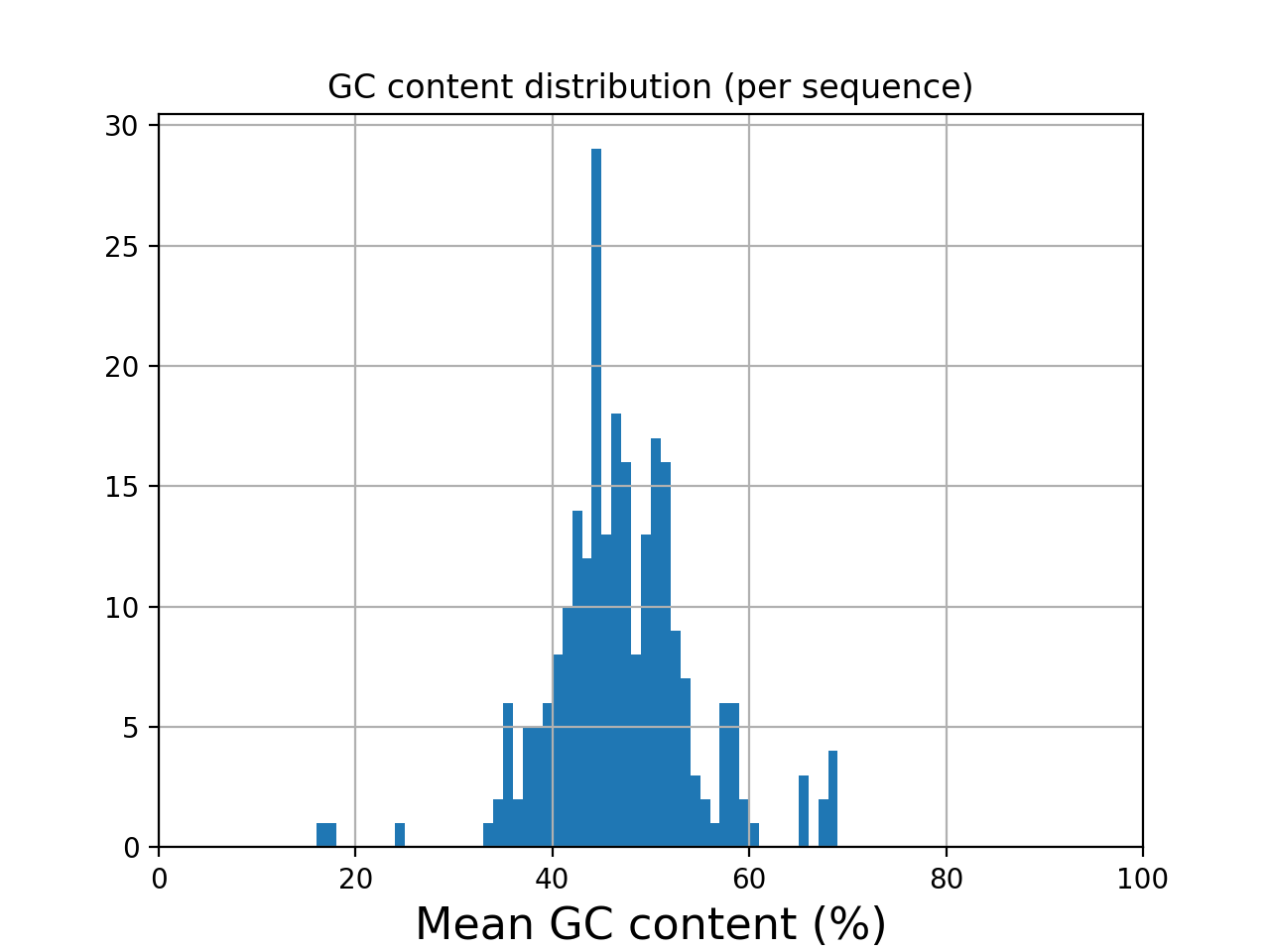
qc.histogram_gc_content()

(Source code, png, hires.png, pdf)

histogram_sequence_lengths(logy=True)

Histogram sequence lengths

from sequana import sequana_data
from sequana import FastQC
filename  = sequana_data("test.fastq", "doc")
qc = FastQC(filename)
qc.histogram_sequence_lengths()

(Source code, png, hires.png, pdf)

plot_acgt_content(stacked=False)

Plot histogram of GC content

from sequana import sequana_data
from sequana import FastQC
filename  = sequana_data("test.fastq", "doc")
qc = FastQC(filename)
qc.plot_acgt_content()

(Source code, png, hires.png, pdf)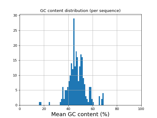

class Identifier(identifier, version='unknown')

Class to interpret Read's identifier

Warning

Implemented for Illumina 1.8+ and 1.4 . Other cases will simply stored the identifier without interpretation

>>> from sequana import Identifier
>>> ident = Identifier('@EAS139:136:FC706VJ:2:2104:15343:197393 1:Y:18:ATCACG')
>>> ident.info['x_coordinate']
'2'

Currently, the following identifiers will be recognised automatically:

Illumina_1_4:

An example is

@HWUSI-EAS100R:6:73:941:1973#0/1

Illumina_1_8:

An example is:

@EAS139:136:FC706VJ:2:2104:15343:197393 1:Y:18:ATCACG

Other that could be implemented are NCBI

@FSRRS4401BE7HA [length=395] [gc=36.46] [flows=800] [phred_min=0]                                            [phred_max=40] [trimmed_length=95]

Information can also be found here http://support.illumina.com/help/SequencingAnalysisWorkflow/Content/Vault/Informatics/Sequencing_Analysis/CASAVA/swSEQ_mCA_FASTQFiles.htm

is_fastq(filename)

11.10. FASTA module

Utilities to manipulate FastA files

class FastA(filename, verbose=False)

Class to handle FastA files

Works like an iterator:

from sequana import FastA
f = FastA("test.fa")
read = next(f)

names and sequences can be accessed with attributes:

f.names
f.sequences

GC_content()

Return GC content in percentage of all sequences found in the FastA file

GC_content_sequence(sequence)

Return GC content in percentage of a sequence

property comments

explode(outdir='.')

extract sequences from one fasta file and save them into individual files

filter(output_filename, names_to_keep=None, names_to_exclude=None)

save FastA excluding or including specific sequences

format_contigs_denovo(output_file, len_min=500)

Remove contigs with sequence length below specific threshold.

Parameters:

• output_file (str) -- output file name.

• len_min (int) -- minimal length of contigs.

Example:

from sequana import FastA

contigs = FastA("denovo_assembly.fasta")
contigs.format_contigs_denovo("output.fasta", len_min=500)

get_lengths_as_dict()

Return dictionary with sequence names and lengths as keys/values

get_stats()

Return a dictionary with basic statistics

N the number of contigs, the N50 and L50, the min/max/mean contig lengths and total length.

property lengths

property names

next()

reverse_and_save(filename)

Reverse sequences and save in a file

save_collapsed_fasta(outfile, ctgname, width=80, comment=None)

Concatenate all contigs and save results

save_ctg_to_fasta(ctgname, outname, max_length=-1)

Select a contig and save in a file

select_random_reads(N=None, output_filename='random.fasta')

Select random reads and save in a file

Parameters:

• N (int) -- number of random unique reads to select should provide a number but a list can be used as well.

• output_filename (str) --

property sequences

summary(max_contigs=-1)

returns summary and print information on the stdout

This method is used when calling sequana standalone

sequana summary test.fasta

to_fasta(outfile, width=80)

Save the input FastA file into a new file

The interest of this method is to wrap the sequence into 80 characters. This is useful if the input file is not formatted correctly.

to_igv_chrom_size(output)

Create a IGV file storing chromosomes and their sizes

11.11. Feature counts module

feature counts related tools

class FeatureCount(filename, clean_sample_names=True, extra_name_rm=['_Aligned'], drop_loc=True, guess_design=False)

Read a featureCounts output file.

The input file is expected to be generated with featurecounts tool. It should be a TSV file such as the following one with the header provided herebelow. Of course input BAM files can be named after your samples:

Geneid    Chr    Start    End    Strand    Length    WT1    WT2 WT3 KO1 KO2 KO3
gene1    NC_010602.1    141    1466    +    1326    11    20    15    13    17    17
gene2    NC_010602.1    1713    2831    +    1119    35    54    58    34    53    46
gene3    NC_010602.1    2831    3934    +    1104    9    16    16    4    18    18

from sequana import FeatureCount
fc = FeatureCount("all_features.out", extra_name_rm=["_S\d+"]
fc.rnadiff_df.to_csv("fc.csv")

Constructor

Get the featureCounts output as a pandas DataFrame

Parameters:

• clean_sample_names (bool) -- if simplifying the sample names in featureCount output columns

• extra_name_rm (list) -- extra list of regex to remove from samples_names (ignored if clean_sample_name is False)

• drop_loc (bool) -- if dropping the extra location columns (ie getting only the count matrix)

property df

class FeatureCountMerger(pattern='*feature.out', fof=[], skiprows=1)

Merge several feature counts files

to_tsv(output_filename='all_features.out')

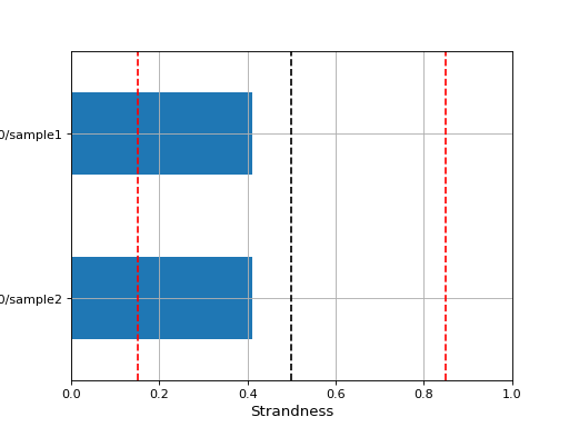
class MultiFeatureCount(rnaseq_folder='.', tolerance=0.1)

Read set of feature counts using different options of strandness

from sequana import sequana_data
from sequana.featurecounts import *
directory = sequana_data("/rnaseq_0")
ff = MultiFeatureCount(directory, 0.15)
ff._get_most_probable_strand_consensus()
ff.plot_strandness()

(Source code, png, hires.png, pdf)

See also

get_most_probable_strand() for more information about the tolerance parameter and meaning of strandness.

The expected data structure is

rnaseq_folder
├── sample1
│   ├── feature_counts_0
│   │   └── sample_feature.out
│   ├── feature_counts_1
│   │   └── sample_feature.out
│   ├── feature_counts_2
│   │   └── sample_feature.out
└── sample2
    ├── feature_counts_0
    │   └── sample_feature.out
    ├── feature_counts_1
    │   └── sample_feature.out
    ├── feature_counts_2
    │   └── sample_feature.out

The new expected data structure is

new_rnaseq_output/
├── sample1
│   └── feature_counts
│       ├── 0
│       │   └── sample_feature.out
│       ├── 1
│       │   └── sample_feature.out
│       └── 2
│           └── sample_feature.out
└── sample2
    └── feature_counts
        ├── 0
        │   └── sample_feature.out
        ├── 1
        │   └── sample_feature.out
        └── 2
            └── sample_feature.out

Parameters:

• rnaseq_folder (str) --

• tolerance (int) -- the tolerance between 0 and 0.25

plot_strandness(fontsize=12, output_filename='strand_summary.png', savefig=False)

get_most_probable_strand(filenames, tolerance, sample_name)

Return most propable strand given 3 feature count files (strand of 0,1, and 2)

Return the total counts by strand from featureCount matrix folder, strandness and probable strand for a single sample (using a tolerance threshold for strandness). This assumes a single sample by featureCounts file.

Parameters:

• filenames -- a list of 3 feature counts files for a given sample corresponding to the strand 0,1,2

• tolerance -- a value below 0.5

• sample -- the name of the sample corresponding to the list in filenames

Possible values returned are:

• 0: unstranded

• 1: stranded

• 2: eversely stranded

We compute the number of counts in case 1 and 2 and compute the ratio strand as . Then we decide on the possible strandness with the following criteria:

• if RS < tolerance, reversely stranded

• if RS in 0.5+-tolerance: unstranded.

• if RS > 1-tolerance, stranded

• otherwise, we cannot decided.

get_most_probable_strand_consensus(rnaseq_folder, tolerance, sample_pattern='*/feature_counts_[012]', file_pattern='feature_counts_[012]/*_feature.out')

From a sequana RNA-seq run folder get the most probable strand, based on the frequecies of counts assigned with '0', '1' or '2' type strandness (featureCounts nomenclature) across all samples.

Parameters:

• rnaseq_folder -- the main directory

• tolerance -- a value in the range 0-0.5. typically 0.1 or 0.15

• pattern -- the samples directory pattern

• pattern_file -- the feature counts pattern

If guess is not possible given the tolerance, fills with None

Consider this tree structure:

rnaseq_folder
├── sample1
│   └── feature_counts
│       ├── 0
│       │   └── sample_feature.out
│       ├── 1
│       │   └── sample_feature.out
│       └── 2
│           └── sample_feature.out
└── sample2
    └── feature_counts
        ├── 0
        │   └── sample_feature.out
        ├── 1
        │   └── sample_feature.out
        └── 2
            └── sample_feature.out

Then, the following command should all files and report the most probable strand (0,1,2) given the sample1 and sample2:

get_most_probable_strand_consensus("rnaseq_folder", 0.15)

This tree structure is understood automatically. If you have a different one, you can set the pattern (for samples) and pattern_files parameters.

11.12. Sequence and genomic modules

class DNA(sequence, codons_stop=['TAA', 'TGA', 'TAG'], codons_stop_rev=['TTA', 'TCA', 'CTA'], codons_start=['ATG'], codons_start_rev=['CAT'])

Simple DNA class

>>> from sequana.sequence import DNA
>>> d = DNA("ACGTTTT")
>>> d.reverse_complement()

Some long computations are done when setting the window size:

d.window = 100

The ORF detection has been validated agains a plasmodium 3D7 ORF file found on plasmodb.org across the 14 chromosomes.

Constructor

A sequence is just a string stored in the sequence attribute. It has properties related to the type of alphabet authorised.

Parameters:

• sequence (str) -- May be a string of a Fasta File, in which case only the first sequence is used.

• complement_in --

• complement_out --

• letters -- authorise letters. Used in check() only.

Todo

use counter only once as a property

property AT_skew

property GC_skew

property ORF_pos

barplot_count_ORF_CDS_by_frame(alpha=0.5, bins=40, xlabel='Frame', ylabel='#', bar_width=0.35)

entropy(sequence)

hist_ORF_CDS_linearscale(alpha=0.5, bins=40, xlabel='Length', ylabel='#')

hist_ORF_CDS_logscale(alpha=0.5, bins=40, xlabel='Length', ylabel='#')

plot_all_skews(figsize=(10, 12), fontsize=16, alpha=0.5)

property threshold

property type_filter

property type_window

property window

class RNA(sequence)

Simple RNA class

>>> from sequana.sequence import RNA
>>> d = RNA("ACGUUUU")
>>> d.reverse_complement()

Constructor

A sequence is just a string stored in the sequence attribute. It has properties related to the type of alphabet authorised.

Parameters:

• sequence (str) -- May be a string of a Fasta File, in which case only the first sequence is used.

• complement_in --

• complement_out --

• letters -- authorise letters. Used in check() only.

Todo

use counter only once as a property

class Repeats(filename_fasta, merge=False, name=None)

Class for finding repeats in DNA or RNA linear sequences.

Computation is performed each time the threshold is set to a new value.

from sequana import sequana_data, Repeats
rr = Repeats(sequana_data("measles.fa"))
rr.threshold = 4
rr.hist_length_repeats()

(Source code)

Note

Works with shustring package from Bioconda (April 2017)

Todo

use a specific sequence (first one by default). Others can be selected by name

Constructor

Input must be a fasta file with valid DNA or RNA characters

Parameters:

• filename_fasta (str) -- a Fasta file, only the first sequence is used !

• threshold (int) -- Minimal length of repeat to output

• name (str) -- if name is provided, scan the Fasta file and select the corresponding sequence. if you want to analyse all sequences, you need to use a loop by setting _header for each sequence with the sequence name found in sequence header.

Note

known problems. Header with a > character (e.g. in the comment) are left strip and only the comments is kept. Another issue is for multi-fasta where one sequence is ignored (last or first ?)

property begin_end_repeat_position

property df_shustring

Return dataframe with shortest unique substring length at each position shortest unique substrings are unique in the sequence and its complement Uses shustring tool

property do_merge

property header

get first line of fasta (needed in input shustring) and replace spaces by underscores

hist_length_repeats(bins=20, alpha=0.5, hold=False, fontsize=12, grid=True, title='Repeat length', xlabel='Repeat length', ylabel='#', logy=True)

Plots histogram of the repeat lengths

property length

property list_len_repeats

property longest_shustring

property names

plot(clf=True)

property threshold

class Sequence(sequence, complement_in=b'ACGT', complement_out=b'TGCA', letters='ACGT')

Abstract base classe for other specialised sequences such as DNA.

Sequenced is the base class for other classes such as DNA and RNA.

from sequana import Sequence
s = Sequence("ACGT")
s.stats()
s.get_complement()

Note

You may use a Fasta file as input (see constructor)

Constructor

A sequence is just a string stored in the sequence attribute. It has properties related to the type of alphabet authorised.

Parameters:

• sequence (str) -- May be a string of a Fasta File, in which case only the first sequence is used.

• complement_in --

• complement_out --

• letters -- authorise letters. Used in check() only.

Todo

use counter only once as a property

check()

Check that all letters are valid

complement()

Alias to get_complement()

gc_content()

Return mean GC content

get_complement()

Return complement

get_occurences(pattern, overlap=False)

Return position of the input pattern in the sequence

>>> from sequana import Sequence
>>> s = Sequence('ACGTTTTACGT')
>>> s.get_occurences("ACGT")
[0, 7]

get_reverse()

Return reverse sequence

get_reverse_complement()

Return reverse complement

reverse()

Alias to get_reverse()

reverse_complement()

Alias to get_reverse_complement

property sequence

stats()

Return basic stats about the number of letters

Utilities to manipulate and find codons

class Codon

Utilities to manipulate codons

The codon contains hard-coded set of start and stop codons (bacteria) for strand plus and minus. Adapt to your needs for other organisms. Based on the scan of Methanothermobacter thermautotrophicus bacteria.

from sequana import Codon
c = Codon()
c.start_codons['+']

codons = {'start': {'+': frozenset({'ATG', 'GTG', 'TTG'}), '-': frozenset({'CAA', 'CAC', 'CAT'})}, 'stop': {'+': frozenset({'TAA', 'TAG', 'TGA'}), '-': frozenset({'CTA', 'TCA', 'TTA'})}}

find_start_codon_position(sequence, position, strand, max_shift=10000)

Return starting position and string of closest start codon to a given position

The starting position is on the 5-3 prime direction (see later)

Parameters:

• sequence (str) --

• position (int) -- 0-base position

• strand (str) -- '+' or '-'

The search starts at the given position, then +1 base, then -1 base, then +2, -2, +3, etc

Here, we start at position 2 (letter G), then shift by +1 and find the ATG string.

>>> from sequana import Codon
>>> c = Codon()
>>> c.find_start_codon_position("ATGATGATG", 2, "+")
(3, 'ATG')

whereas starting at position 1, a shift or +1 (position 2 ) does not hit a start codon. Next, a shift of -1 (position 0) hits the ATG start codon.:

>>> c.find_start_codon_position("ATGATGATG", 1, "+")
(3, 'ATG')

On strand -, the start codon goes from right to left. So, in the following example, the CAT start codon (reverse complement of ATG) is found at position 3. Developers must take into account a +3 shift if needed:

>>> c.find_start_codon_position("AAACAT", 3, "-")
(3, 'CAT')

>>> c.find_start_codon_position("AAACATCAT", 8, "-")

find_stop_codon_position(sequence, position, strand, max_shift=10000)

Return position and string of closest stop codon to a given position

Parameters:

• sequence (str) --

• position (int) -- 0-base position

• strand (str) --

  • or -

See find_start_codon_position() for details.

Only difference is that the search is based on stop codons rather than start codons.

>>> from sequana import Codon
>>> c = Codon()
>>> c.find_stop_codon_position("ATGACCCC", 2, "+")
(1, 'TGA')

get_codons_from_fasta_and_gff(fasta, gff)

11.13. Kmer module

build_kmer(length=6, letters='CG')

Return list of kmer of given length based on a set of letters

Returns:

list of kmers

get_kmer(sequence, k=7)

Given a sequence, return consecutive kmers

Returns:

iterator of kmers

11.14. Taxonomy related (Kraken - Krona)

class KrakenAnalysis(fastq, database, threads=4, confidence=0)

Run kraken on a set of FastQ files

In order to run a Kraken analysis, we firtst need a local database. We provide a Toy example. The ToyDB is downloadable as follows ( you will need to run the following code only once):

from sequana import KrakenDownload
kd = KrakenDownload()
kd.download_kraken_toydb()

See also

KrakenDownload for more databases

The path to the database is required to run the analysis. It has been stored in the directory ./config/sequana/kraken_toydb under Linux platforms The following code should be platform independent:

import os
from sequana import sequana_config_path
database = sequana_config_path + os.sep + "kraken_toydb")

Finally, we can run the analysis on the toy data set:

from sequana import sequana_data
data = sequana_data("Hm2_GTGAAA_L005_R1_001.fastq.gz", "data")
ka = KrakenAnalysis(data, database=database)
ka.run()

This creates a file named kraken.out. It can be interpreted with KrakenResults

Constructor

Parameters:

• fastq -- either a fastq filename or a list of 2 fastq filenames

• database -- the path to a valid Kraken database

• threads -- number of threads to be used by Kraken

• confidence -- parameter used by kraken2

• return --

run(output_filename=None, output_filename_classified=None, output_filename_unclassified=None, only_classified_output=False)

Performs the kraken analysis

Parameters:

• output_filename (str) -- if not provided, a temporary file is used and stored in kraken_output.

• output_filename_classified (str) -- not compressed

• output_filename_unclassified (str) -- not compressed

class KrakenDB(filename)

Class to handle a kraken DB

property version

class KrakenPipeline(fastq, database, threads=4, output_directory='kraken', dbname=None, confidence=0)

Used by the standalone application sequana_taxonomy

This runs Kraken on a set of FastQ files, transform the results in a format compatible for Krona, and creates a Krona HTML report.

from sequana import KrakenPipeline
kt = KrakenPipeline(["R1.fastq.gz", "R2.fastq.gz"], database="krakendb")
kt.run()
kt.show()

Warning

We do not provide Kraken database within sequana. You may either download a database from https://ccb.jhu.edu/software/kraken/ or use this class to download a toy example that will be stored in e.g .config/sequana under Unix platforms. See KrakenDownload.

See also

We provide a standalone application of this class, which is called sequana_taxonomy and can be used within a command shell.

Constructor

Parameters:

• fastq -- either a fastq filename or a list of 2 fastq filenames

• database -- the path to a valid Kraken database

• threads -- number of threads to be used by Kraken

• output_directory -- output filename of the Krona HTML page

• dbname --

Description: internally, once Kraken has performed an analysis, reads are associated to a taxon (or not). We then find the correponding lineage and scientific names to be stored within a Krona formatted file. KtImportTex is then used to create the Krona page.

run(output_filename_classified=None, output_filename_unclassified=None, only_classified_output=False)

Run the analysis using Kraken and create the Krona output

Todo

reuse the KrakenResults code to simplify this method.

show()

Opens the filename defined in the constructor

class KrakenResults(filename='kraken.out', verbose=True)

Translate Kraken results into a Krona-compatible file

If you run a kraken analysis with KrakenAnalysis, you will end up with a file e.g. named kraken.out (by default).

You could use kraken-translate but then you need extra parsing to convert into a Krona-compatible file. Here, we take the output from kraken and directly transform it to a krona-compatible file.

kraken2 uses the --use-names that needs extra parsing.

k = KrakenResults("kraken.out")
k.kraken_to_krona()

Then format expected looks like:

C    HISEQ:426:C5T65ACXX:5:2301:18719:16377    1    203    1:71 A:31 1:71
C    HISEQ:426:C5T65ACXX:5:2301:21238:16397    1    202    1:71 A:31 1:71

Where each row corresponds to one read.

"562:13 561:4 A:31 0:1 562:3" would indicate that:

the first 13 k-mers mapped to taxonomy ID #562
the next 4 k-mers mapped to taxonomy ID #561
the next 31 k-mers contained an ambiguous nucleotide
the next k-mer was not in the database
the last 3 k-mers mapped to taxonomy ID #562

For kraken2, format is slighlty different since it depends on paired or not. If paired,

C   read1 2697049 151|151 2697049:117 |:| 0:1 2697049:116

See kraken documentation for details.

Note

a taxon of ID 1 (root) means that the read is classified but in differen domain. https://github.com/DerrickWood/kraken/issues/100

Note

This takes care of fetching taxons and the corresponding lineages from online web services.

constructor

Parameters:

filename -- the input from KrakenAnalysis class

boxplot_classified_vs_read_length()

Show distribution of the read length grouped by classified or not

property df

get_taxonomy_db(ids)

Retrieve taxons given a list of taxons

Parameters:

ids (list) -- list of taxons as strings or integers. Could also be a single string or a single integer

Returns:

a dataframe

Note

the first call first loads all taxons in memory and takes a few seconds but subsequent calls are much faster

histo_classified_vs_read_length()

Show distribution of the read length grouped by classified or not

kraken_to_csv(filename, dbname)

kraken_to_json(filename, dbname)

kraken_to_krona(output_filename=None, nofile=False)

Returns:

status: True is everything went fine otherwise False

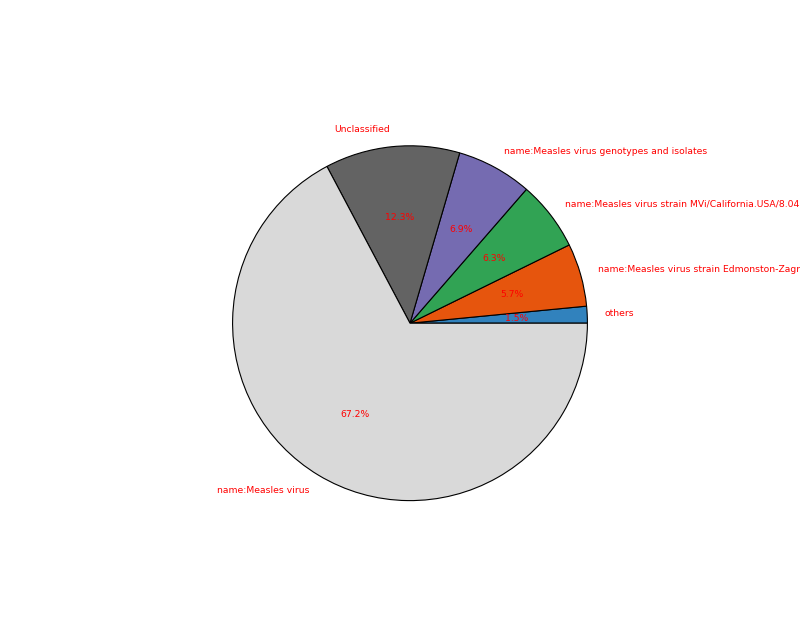
plot(kind='pie', cmap='tab20c', threshold=1, radius=0.9, textcolor='red', delete_krona_file=False, **kargs)

A simple non-interactive plot of taxons

Returns:

None if no taxon were found and a dataframe otherwise

A Krona Javascript output is also available in kraken_to_krona()

from sequana import KrakenResults, sequana_data
test_file = sequana_data("kraken.out", "doc")
k = KrakenResults(test_file)
df = k.plot(kind='pie')

(Source code, png, hires.png, pdf)

See also

to generate the data see KrakenPipeline or the standalone application sequana_taxonomy.

Todo

For a future release, we could use this kind of plot https://stackoverflow.com/questions/57720935/how-to-use-correct-cmap-colors-in-nested-pie-chart-in-matplotlib

plot2(kind='pie', fontsize=12)

This is the simplified static krona-like plot included in HTML reports

property taxons

to_js(output='krona.html')

class KrakenSequential(filename_fastq, fof_databases, threads=1, output_directory='./kraken_sequential/', keep_temp_files=False, output_filename_unclassified=None, output_filename_classified=None, force=False, confidence=0)

Kraken Sequential Analysis

This runs Kraken on a FastQ file with multiple k-mer databases in a sequencial way way. Unclassified sequences with the first database are input for the second, and so on.

The input may be a single FastQ file or paired, gzipped or not. FastA are also accepted.

constructor

Parameters:

• filename_fastq -- FastQ file to analyse

• fof_databases -- file that contains a list of databases paths (one per line). The order is important. Note that you may also provide a list of datab ase paths.

• threads -- number of threads to be used by Kraken

• output_directory -- name of the output directory

• keep_temp_files -- bool, if True, will keep intermediate files from each Kraken analysis, and save html report at each step

• force (bool) -- if the output directory already exists, the instanciation fails so that the existing data is not overrwritten. If you wish to overwrite the existing directory, set this parameter to iTrue.

run(dbname='multiple', output_prefix='kraken_final')

Run the sequential analysis

Parameters:

• dbname --

• output_prefix --

Returns:

dictionary summarizing the databases names and classified/unclassied

This method does not return anything creates a set of files:

• kraken_final.out

• krona_final.html

• kraken.png (pie plot of the classified/unclassified reads)

Note

the databases are run in the order provided in the constructor.

class MultiKrakenResults(filenames, sample_names=None)

Select several kraken output and creates summary plots

import glob
mkr = MultiKrakenResults(glob.glob("*/*/kraken.csv"))
mkr.plot_stacked_hist()

get_df(limit=5, rank='kingdom')

plot_stacked_hist(output_filename=None, dpi=200, kind='barh', fontsize=10, edgecolor='k', lw=1, width=1, ytick_fontsize=10, max_labels=50, max_sample_name_length=30, rank='kingdom')

Summary plot of reads classified.

class MultiKrakenResults2(filenames, sample_names=None)

Select several kraken output and creates summary plots

import glob
mkr = MultiKrakenResults2(glob.glob("*/*/summary.json"))
mkr.plot_stacked_hist()

get_df(limit=5, sorting_method='sample_name')

plot_stacked_hist(output_filename=None, dpi=200, kind='barh', fontsize=10, edgecolor='k', lw=2, width=1, ytick_fontsize=10, max_labels=50, alpha=0.8, colors=None, cmap='viridis', sorting_method='sample_name', max_sample_name_length=30)

Summary plot of reads classified.

Parameters:

• sorting_method -- only by sample name for now

• cmap -- a valid matplotlib colormap. viridis is the default sequana colormap.

if you prefer to use a colormap, you can use:

from matplotlib import cm
cm = matplotlib.colormap
colors = [cm.get_cmap(cmap)(x) for x in pylab.linspace(0.2, 1, L)]

class NCBITaxonomy(names, nodes)

Parameters:

• names -- can be a local file or URL

• nodes -- can be a local file or URL

create_taxonomy_file(filename='taxonomy.csv.gz')

class Taxonomy(*args, **kwargs)

This class should ease the retrieval and manipulation of Taxons

There are many resources to retrieve information about a Taxon. For instance, from BioServices, one can use UniProt, Ensembl, or EUtils. This is convenient to retrieve a Taxon (see fetch_by_name() and fetch_by_id() that rely on Ensembl). However, you can also download a flat file from EBI ftp server, which stores a set or records (2.8M (april 2020).

Note that the Ensembl database does not seem to be as up to date as the flat files but entries contain more information.

for instance taxon 2 is in the flat file but not available through the fetch_by_id(), which uses ensembl.

So, you may access to a taxon in 2 different ways getting differnt dictionary. However, 3 keys are common (id, parent, scientific_name)

>>> t = taxonomy.Taxonomy()
>>> t.fetch_by_id(9606)   # Get a dictionary from Ensembl
>>> t.records[9606] # or just try with the get
>>> t[9606]
>>> t.get_lineage(9606)

Possible ranks are various. You may have biotype, clade, etc ub generally speaking ranks are about lineage. For a given rank, e.g. kingdom, you may have sub division such as superkingdom and subkingdom. order has even more subdivisions (infra, parv, sub, super)

Since version 0.8.3 we use NCBI that is updated more often than the ebi ftp according to their README. ftp://ncbi.nlm.nih.gov/pub/taxonomy/ We use Ensembl to retrieve various information regarding taxons.

constructor

Parameters:

• offline -- if you do not have internet, the connction to Ensembl may hang for a while and fail. If so, set offline to True

• from -- download taxonomy databases from ncbi

download_taxonomic_file(overwrite=False)

Loads entire flat file from NCBI

Do not overwrite the file by default.

fetch_by_id(taxon)

Search for a taxon by identifier

:return; a dictionary.

>>> ret = s.search_by_id('10090')
>>> ret['name']
'Mus Musculus'

fetch_by_name(name)

Search a taxon by its name.

Parameters:

name (str) -- name of an organism. SQL cards possible e.g., _ and % characters.

Returns:

a list of possible matches. Each item being a dictionary.

>>> ret = s.search_by_name('Mus Musculus')
>>> ret[0]['id']
10090

find_taxon(taxid, mode='ncbi')

get_children(taxon)

get_lineage(taxon)

Get lineage of a taxon

Parameters:

taxon (int) -- a known taxon

Returns:

list containing the lineage

get_lineage_and_rank(taxon)

Get lineage and rank of a taxon

Parameters:

taxon (int) --

Returns:

a list of tuples. Each tuple is a pair of taxon name/rank The list is the lineage for to the input taxon.

get_names_for_given_rank(rank)

get_parent_name(taxon)

get_parent_taxon(taxon)

get_ranks()

get_records_for_given_rank(rank)

load_records(overwrite=False)

Load a flat file and store records in records

load_records_from_csv(filename)

11.15. Pacbio module

Pacbio QC and stats

class BAMSimul(filename)

BAM reader for Pacbio simulated reads (PBsim)

A summary of the data is stored in the attribute df. It contains information such as the length of the reads, the ACGT content, the GC content.

Constructor

Parameters:

filename (str) -- filename of the input pacbio BAM file. The content of the BAM file is not the ouput of a mapper. Instead, it is the output of a Pacbio (Sequel) sequencing (e.g., subreads).

property df

filter_bool(output_filename, mask)

Select and Write reads using a mask

Parameters:

• output_filename (str) -- name of output file

• list_bool (list) -- True to write read to output, False to ignore it

filter_length(output_filename, threshold_min=0, threshold_max=inf)

Select and Write reads within a given range

Parameters:

• output_filename (str) -- name of output file

• threshold_min (int) -- minimum length of the reads to keep

• threshold_max (int) -- maximum length of the reads to keep

hist_GC(bins=50, alpha=0.5, hold=False, fontsize=12, grid=True, xlabel='GC %', ylabel='#', label='', title=None)

Plot histogram GC content

Parameters:

• bins (int) -- binning for the histogram

• alpha (float) -- transparency of the histograms

• hold (bool) --

• fontsize (int) -- fontsize of the x and y labels and title.

• grid (bool) -- add grid or not

• xlabel (str) --

• ylabel (str) --

• label (str) -- label of the histogram (for the legend)

• title (str) --

from sequana.pacbio import PacbioSubreads
from sequana import sequana_data
b = PacbioSubreads(sequana_data("test_pacbio_subreads.bam"))
b.hist_GC()

(Source code, png, hires.png, pdf)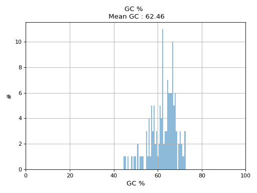

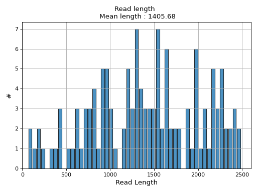
hist_read_length(bins=50, alpha=0.8, hold=False, fontsize=12, grid=True, xlabel='Read Length', ylabel='#', label='', title=None, logy=False, ec='k', hist_kwargs={})

Plot histogram Read length

Parameters:

• bins (int) -- binning for the histogram

• alpha (float) -- transparency of the histograms

• hold (bool) --

• fontsize (int) --

• grid (bool) --

• xlabel (str) --

• ylabel (str) --

• label (str) -- label of the histogram (for the legend)

• title (str) --

from sequana.pacbio import PacbioSubreads
from sequana import sequana_data
b = PacbioSubreads(sequana_data("test_pacbio_subreads.bam"))
b.hist_read_length()

(Source code, png, hires.png, pdf)

plot_GC_read_len(hold=False, fontsize=12, bins=[200, 60], grid=True, xlabel='GC %', ylabel='#', cmap='BrBG')

Plot GC content versus read length

Parameters:

• hold (bool) --

• fontsize (int) -- for x and y labels and title

• bins -- a integer or tuple of 2 integers to specify the binning of the x and y 2D histogram.

• grid (bool) --

• xlabel (str) --

• ylabel (str) --

from sequana.pacbio import PacbioSubreads
from sequana import sequana_data
b = PacbioSubreads(sequana_data("test_pacbio_subreads.bam"))
b.plot_GC_read_len(bins=[10, 10])

(Source code, png, hires.png, pdf)

reset()

to_fasta(output_filename, threads=2)

Export BAM reads into a Fasta file

Parameters:

• output_filename -- name of the output file (use .fasta extension)

• threads (int) -- number of threads to use

Note

this executes a shell command based on samtools

Warning

this takes a few minutes for 500,000 reads

to_fastq(output_filename, threads=2)

Export BAM reads into FastQ file

class Barcoding(filename)

Read as input a file created by smrtlink that stores statistics about each barcode. This is a simple CSV file with one line per barcode<

hist_mean_polymerase_read_length(bins=10, fontsize=12)

hist_polymerase_per_barcode(bins=10, fontsize=12)

histogram of number of polymerase per barcode

Cumulative histogram gives total number of polymerase reads

hist_quality_per_barcode(bins=10, fontsize=12)

plot_and_save_all(dpi=100, directory='.')

plot_polymerase_per_barcode(fontsize=12, unbarcoded=True)

Number Of Polymerase Reads Per Barcode

plot_subreads_histogram(bins=10, fontsize=12)

class PBSim(input_bam, simul_bam)

Filter an input BAM (simulated with pbsim) so as so keep reads that fit a target distribution.

This uses a MH algorithm behind the scene.

ss = pacbio.PBSim("test10X.bam")
clf();
ss.run(bins=100, step=50)

For example, to simulate data set, use:

pbsim --data-type CLR --accuracy-min 0.85 --depth 20              --length-mean 8000 --length-sd 800 reference.fasta --model_qc model_qc_clr

The file model_qc_clr can be retrieved from the github here below.

See https://github.com/pfaucon/PBSIM-PacBio-Simulator for details.

We get a fastq file where simulated read sequences are randomly sampled from the reference sequence ("reference.fasta") and differences (errors) of the sampled reads are introduced.

The Fastq can be converted to

run(bins=50, xmin=0, xmax=30000, step=1000, burn=1000, alpha=1, output_filename=None)

target_distribution(xprime)

The target distribution

Compute histogram. Get X, Y. Given xprime, interpolate to get yprime use e.g. np.interp

class PacbioMappedBAM(filename, method)

Parameters:

filename (str) -- input BAM file

boxplot_mapq_concordance()

filter_mapq(output_filename, threshold_min=0, threshold_max=255)

Select and Write reads within a given range

Parameters:

• output_filename (str) -- name of output file

• threshold_min (int) -- minimum length of the reads to keep

• threshold_max (int) -- maximum length of the reads to keep

get_coverage(reference_length=None)

hist_GC(bins=50, alpha=0.5, hold=False, fontsize=12, grid=True, xlabel='GC %', ylabel='#', label='', title=None)

Plot histogram GC content

Parameters:

• bins (int) -- binning for the histogram

• alpha (float) -- transparency of the histograms

• hold (bool) --

• fontsize (int) -- fontsize of the x and y labels and title.

• grid (bool) -- add grid or not

• xlabel (str) --

• ylabel (str) --

• label (str) -- label of the histogram (for the legend)

• title (str) --

from sequana.pacbio import PacbioSubreads
from sequana import sequana_data
b = PacbioSubreads(sequana_data("test_pacbio_subreads.bam"))
b.hist_GC()

(Source code, png, hires.png, pdf)

hist_concordance(bins=100, fontsize=16)

formula : 1 - (in + del + mismatch / (in + del + mismatch + match) )

For BWA and BLASR, the get_cigar_stats are different !!! BWA for instance has no X stored while Pacbio forbids the use of the M (CMATCH) tag. Instead, it uses X (CDIFF) and = (CEQUAL) characters.

Subread Accuracy: The post-mapping accuracy of the basecalls. Formula: [1 - (errors/subread length)], where errors = number of deletions + insertions + substitutions.

hist_median_ccs(bins=1000, **kwargs)

Group subreads by ZMW and plot median of read length for each polymerase

hist_read_length(bins=50, alpha=0.8, hold=False, fontsize=12, grid=True, xlabel='Read Length', ylabel='#', label='', title=None, logy=False, ec='k', hist_kwargs={})

Plot histogram Read length

Parameters:

• bins (int) -- binning for the histogram

• alpha (float) -- transparency of the histograms

• hold (bool) --

• fontsize (int) --

• grid (bool) --

• xlabel (str) --

• ylabel (str) --

• label (str) -- label of the histogram (for the legend)

• title (str) --

from sequana.pacbio import PacbioSubreads
from sequana import sequana_data
b = PacbioSubreads(sequana_data("test_pacbio_subreads.bam"))
b.hist_read_length()

(Source code, png, hires.png, pdf)

plot_GC_read_len(hold=False, fontsize=12, bins=[200, 60], grid=True, xlabel='GC %', ylabel='#', cmap='BrBG')

Plot GC content versus read length

Parameters:

• hold (bool) --

• fontsize (int) -- for x and y labels and title

• bins -- a integer or tuple of 2 integers to specify the binning of the x and y 2D histogram.

• grid (bool) --

• xlabel (str) --

• ylabel (str) --

from sequana.pacbio import PacbioSubreads
from sequana import sequana_data
b = PacbioSubreads(sequana_data("test_pacbio_subreads.bam"))
b.plot_GC_read_len(bins=[10, 10])

(Source code, png, hires.png, pdf)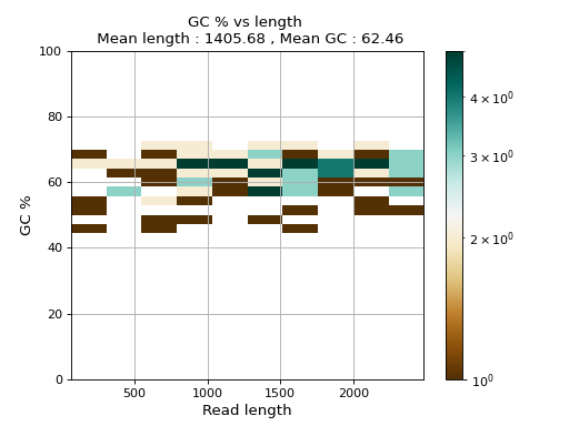

reset()

to_fasta(output_filename, threads=2)

Export BAM reads into a Fasta file

Parameters:

• output_filename -- name of the output file (use .fasta extension)

• threads (int) -- number of threads to use

Note

this executes a shell command based on samtools

Warning

this takes a few minutes for 500,000 reads

to_fastq(output_filename, threads=2)

Export BAM reads into FastQ file

class PacbioSubreads(filename, sample=0)

BAM reader for Pacbio (reads)

You can read a file as follows:

from sequana.pacbio import Pacbiosubreads
from sequana import sequana_data
filename = sequana_data("test_pacbio_subreads.bam")
b = PacbioSubreads(filename)

A summary of the data is stored in the attribute df. It contains information such as the length of the reads, the ACGT content, the GC content.

Several plotting methods are available. For instance, hist_snr().

The BAM file used to store the Pacbio reads follows the BAM/SAM specification. Note that the sequence read are termed query, a subsequence of an entire Pacbio ZMW read ( a subread), which is basecalls from a single pass of the insert DNA molecule.

In general, only a subsequence of the query will align to the reference genome, and that subsequence is referred to as the aligned query.

When introspecting the aligned BAM file, the extent of the query in ZMW read is denoted as [qStart, qEnd) and the extent of the aligned subinterval as [aStart, aEnd). The following graphic illustrates these intervals:

      qStart                         qEnd
0         |  aStart                aEnd  |
[--...----*--*---------------------*-----*-----...------)  < "ZMW read" coord. system
          ~~~----------------------~~~~~~                  <  query; "-" =aligning subseq.
[--...-------*---------...---------*-----------...------)  < "ref." / "target" coord. system
0            tStart                tEnd

In the BAM files, the qStart, qEnd are contained in the qs and qe tags, (and reflected in the QNAME); the bounds of the aligned query in the ZMW read can be determined by adjusting qs and qe by the number of soft-clipped bases at the ends of the alignment (as found in the CIGAR).

See also the comments in the code for other tags.

Reference:

http://pacbiofileformats.readthedocs.io/en/3.0/BAM.html

Constructor

Parameters:

• filename (str) -- filename of the input pacbio BAM file. The content of the BAM file is not the ouput of a mapper. Instead, it is the output of a Pacbio (Sequel) sequencing (e.g., subreads).

• sample (int) -- for sample, you can set the number of subreads to read (0 means read all subreads)

boxplot_read_length_vs_passes(nmax=20, ax=None, whis=1.5, widths=0.6)

property df

filter_length(output_filename, threshold_min=0, threshold_max=inf)

Select and Write reads within a given range

Parameters:

• output_filename (str) -- name of output file

• threshold_min (int) -- minimum length of the reads to keep

• threshold_max (int) -- maximum length of the reads to keep

get_mean_nb_passes(min_length=50, max_length=1500000)

get_number_of_ccs(min_length=50, max_length=15000)

hist_GC(bins=50, alpha=0.5, hold=False, fontsize=12, grid=True, xlabel='GC %', ylabel='#', label='', title=None)

Plot histogram GC content

Parameters:

• bins (int) -- binning for the histogram

• alpha (float) -- transparency of the histograms

• hold (bool) --

• fontsize (int) -- fontsize of the x and y labels and title.

• grid (bool) -- add grid or not

• xlabel (str) --

• ylabel (str) --

• label (str) -- label of the histogram (for the legend)

• title (str) --

from sequana.pacbio import PacbioSubreads
from sequana import sequana_data
b = PacbioSubreads(sequana_data("test_pacbio_subreads.bam"))
b.hist_GC()

(Source code, png, hires.png, pdf)

hist_nb_passes(bins=None, alpha=0.8, hold=False, fontsize=12, grid=True, xlabel='Number of passes', logy=True, ec='k', ylabel='#', label='', title='Number of passes')

Plot histogram of number of passes

Parameters:

• alpha (float) -- transparency of the histograms

• hold (bool) --

• fontsize (int) --

• grid (bool) --

• xlabel (str) --

• ylabel (str) --

• logy (bool) -- use log scale on the y axis (default to True)

• label (str) -- label of the histogram (for the legend)

• title (str) --

from sequana.pacbio import PacbioSubreads
from sequana import sequana_data
b = PacbioSubreads(sequana_data("test_pacbio_subreads.bam"))
b.hist_nb_passes()

(Source code, png, hires.png, pdf)

hist_read_length(bins=50, alpha=0.8, hold=False, fontsize=12, grid=True, xlabel='Read Length', ylabel='#', label='', title=None, logy=False, ec='k', hist_kwargs={})

Plot histogram Read length

Parameters:

• bins (int) -- binning for the histogram

• alpha (float) -- transparency of the histograms

• hold (bool) --

• fontsize (int) --

• grid (bool) --

• xlabel (str) --

• ylabel (str) --

• label (str) -- label of the histogram (for the legend)

• title (str) --

from sequana.pacbio import PacbioSubreads
from sequana import sequana_data
b = PacbioSubreads(sequana_data("test_pacbio_subreads.bam"))
b.hist_read_length()

(Source code, png, hires.png, pdf)

hist_snr(bins=50, alpha=0.5, hold=False, fontsize=12, grid=True, xlabel='SNR', ylabel='#', title='', clip_upper_SNR=30)

Plot histogram of the ACGT SNRs for all reads

Parameters:

• bins (int) -- binning for the histogram. Note that the range starts at 0 and ends at clip_upper_SNR

• alpha (float) -- transparency of the histograms

• hold (bool) --

• fontsize (int) --

• grid (bool) --

• xlabel (str) --

• ylabel (str) --

• title (str) --

from sequana.pacbio import PacbioSubreads
from sequana import sequana_data
b = PacbioSubreads(sequana_data("test_pacbio_subreads.bam"))
b.hist_snr()

(Source code, png, hires.png, pdf)

plot_GC_read_len(hold=False, fontsize=12, bins=[200, 60], grid=True, xlabel='GC %', ylabel='#', cmap='BrBG')

Plot GC content versus read length

Parameters:

• hold (bool) --

• fontsize (int) -- for x and y labels and title

• bins -- a integer or tuple of 2 integers to specify the binning of the x and y 2D histogram.

• grid (bool) --

• xlabel (str) --

• ylabel (str) --

from sequana.pacbio import PacbioSubreads
from sequana import sequana_data
b = PacbioSubreads(sequana_data("test_pacbio_subreads.bam"))
b.plot_GC_read_len(bins=[10, 10])

(Source code, png, hires.png, pdf)

random_selection(output_filename, nreads=None, expected_coverage=None, reference_length=None, read_lengths=None)

Select random reads

Parameters:

• nreads -- number of reads to select randomly. Must be less than number of available reads in the orignal file.

• expected_coverage --

• reference_length --

if expected_coverage and reference_length provided, nreads is replaced automatically.

Note

to speed up computation (if you need to call random_selection many times), you can provide the mean read length manually

reset()

save_summary(filename)

property stats

return basic stats about the read length

stride(output_filename, stride=10, shift=0, random=False)

Write a subset of reads to BAM output

Parameters:

• output_filename (str) -- name of output file

• stride (int) -- optionnal, number of reads to read to output one read

• shift (int) -- number of reads to ignore at the begining of input file

• random (bool) -- if True, at each step the read to output is randomly selected

summary()

to_fasta(output_filename, threads=2)

Export BAM reads into a Fasta file

Parameters:

• output_filename -- name of the output file (use .fasta extension)

• threads (int) -- number of threads to use

Note

this executes a shell command based on samtools

Warning

this takes a few minutes for 500,000 reads

to_fastq(output_filename, threads=2)

Export BAM reads into FastQ file

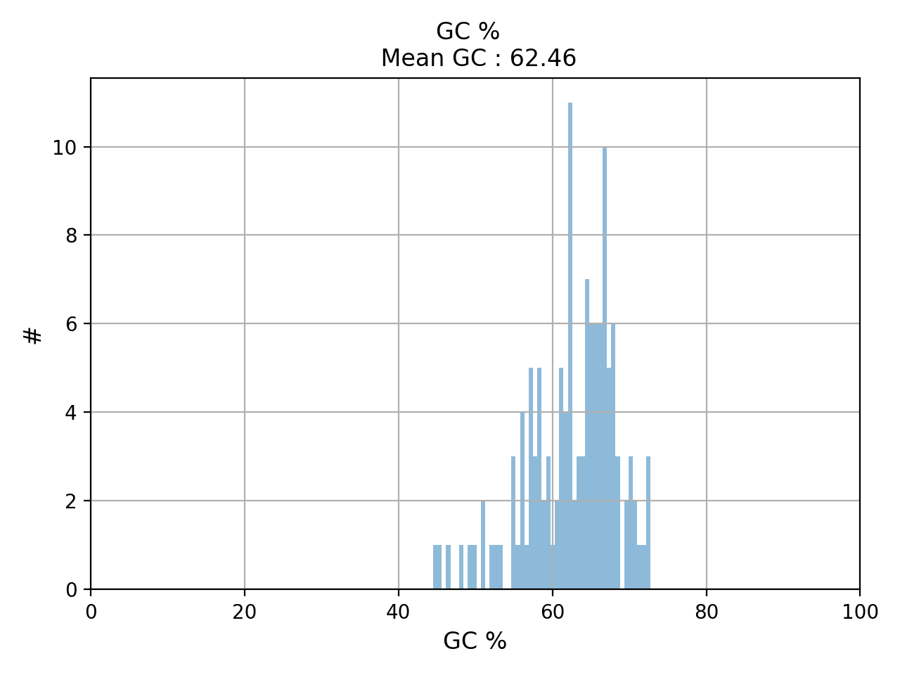
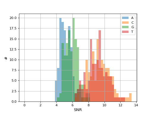
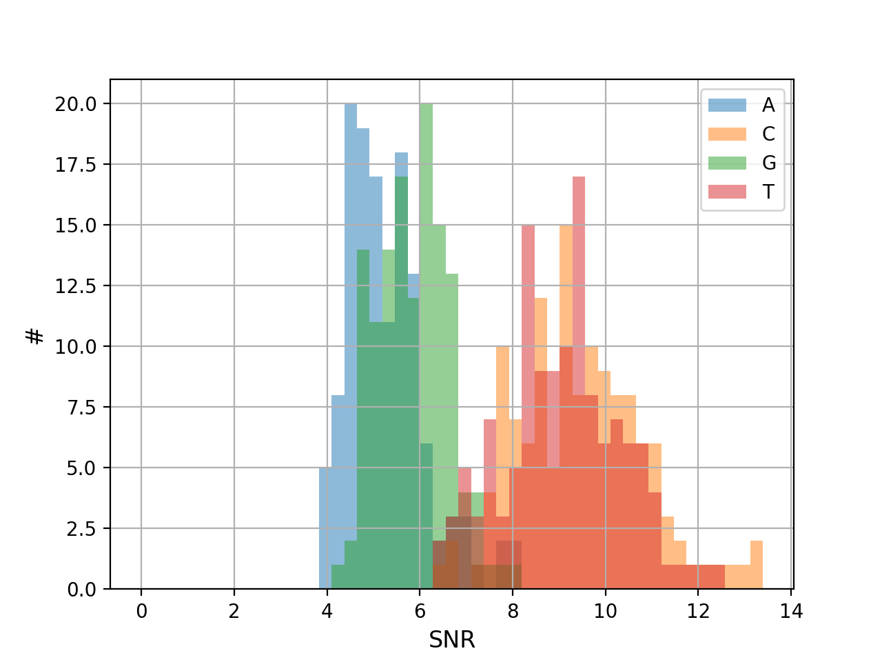
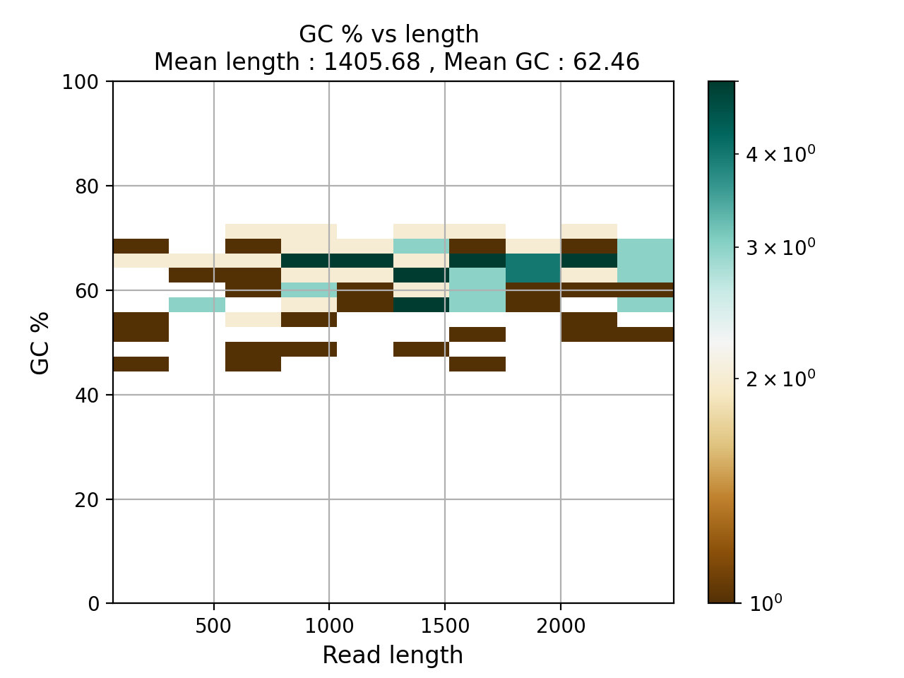
11.16. Phred quality

Manipulate phred quality of reads

FastQ quality are stored as characters. The phred scales indicates the range of characters.

In general, characters goes from ! to ~ that is from 33 to 126 in an ascii table. This convention starts at 33 because characters before ! may cause trouble (e.g. white spaces). This scale is the Sanger scale. There are 2 other scales that could be used ranging from 59 to 126 (illumina 1) and from 64 to 126 (illumina 1.3+).

So, here are the offset to use:

Name	offset	Numeric range
Sanger	33	0 to 93
Solexa	64	-5 to 62
illumina1.3+	64	0 to 62

reference:

http://www.ncbi.nlm.nih.gov/pmc/articles/PMC2847217/

Even though dedicated tools would have better performances, we provide a set of convenient functions. An example is provided here below to plot the quality corresponding to a character string extracted from a FastQ read.

In this example, we use Quality class where the default offset is 33 (Sanger). We compare the quality for another offset

from sequana import phred

from sequana.phred import Quality
q = Quality('BCCFFFFFHHHHHIIJJJJJJIIJJJJJJJJFH')
q.plot()
q.offset = 64
q.plot()
from pylab import legend
legend(loc="best")

(Source code, png, hires.png, pdf)

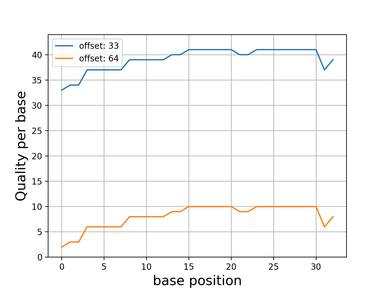
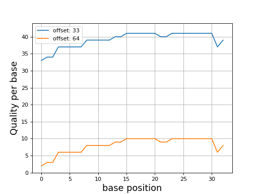
class Quality(seq, offset=33)

Phred quality

>>> from sequana.phred import Quality
>>> q = Quality('BCCFFFFFHHHHHIIJJJJJJIIJJJJJJJJFH')
>>> q.plot()

(Source code, png, hires.png, pdf)

You can access to the quality as a list using the quality attribute and the mean quality from the mean_quality attribute.

property mean_quality

return mean quality

plot(fontsize=16)

plot quality versus base position

property quality

phred string into quality list

proba_to_quality_sanger(pe)

A value between 0 and 93

Parameters:

pe -- the probability of error.

Returns:

Q is the quality score.

• a high probability of error (0.99) gives Q=0

• q low proba of errors (0.05) gives Q = 13

• q low proba of errors (0.01) gives Q = 20

quality_to_proba_sanger(quality)

Quality to probability (Sanger)

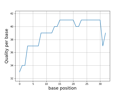
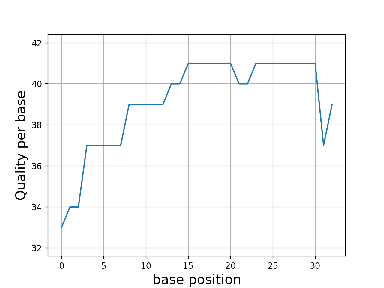
11.17. RiboDesigner

Ribodesigner module

class RiboDesigner(fasta, gff, output_directory, seq_type='rRNA', max_n_probes=384, force=False, threads=4, identity_step=0.01, **kwargs)

Design probes for ribosomes depletion.

From a complete genome assembly FASTA file and a GFF annotation file:

• Extract genomic sequences corresponding to the selected seq_type.

• For these selected sequences, design probes computing probe length and inter probe space according to the length of the ribosomale sequence.

• Detect the highest cd-hit-est identity threshold where the number of probes is inferior or equal to max_n_probes.

• Report the list of probes in BED and CSV files.

In the CSV, the oligo names are in column 1 and the oligo sequences in column 2.

Parameters:

• fasta -- The FASTA file with complete genome assembly to extract ribosome sequences from.

• gff -- GFF annotation file of the genome assembly.

• output_directory -- The path to the output directory.

• seq_type -- string describing sequence annotation type (column 3 in GFF) to select rRNA from.

• max_n_probes -- Max number of probes to design

• force -- If the output_directory already exists, overwrite it.

• threads -- Number of threads to use in cd-hit clustering.

• identity_step (float) -- step to scan the sequence identity (between 0 and 1) defaults to 0.01.

cluster_probes()

Use cd-hit-est to cluster highly similar probes.

clustering_needed(force=False)

Checks if a clustering is needed.

Parameters:

force -- force clustering even if unecessary.

export_to_csv_bed()

Export final results to CSV and BED files

export_to_fasta()

From the self.probes_df, export to FASTA and CSV files.

export_to_json()

get_all_probes(method='original')

Run all probe design and concatenate results in a single DataFrame.

get_rna_pos_from_gff()

Convert a GFF file into a pandas DataFrame filtered according to the self.seq_type.

run(method='greedy')

11.18. RNAdiff

class RNADesign(filename, sep='\\s*,\\s*', condition_col='condition', reference=None)

Simple RNA design handler

checker()

property comparisons

property conditions

keep_conditions(conditions)

validate()

class RNADiffAnalysis(counts_file, design_file, condition, keep_all_conditions=False, reference=None, comparisons=None, batch=None, fit_type='parametric', beta_prior=False, independent_filtering=True, cooks_cutoff=None, gff=None, fc_attribute=None, fc_feature=None, annot_cols=None, threads=4, outdir='rnadiff', sep_counts=',', sep_design='\\s*,\\s*', minimum_mean_reads_per_gene=0, minimum_mean_reads_per_condition_per_gene=0, model=None)

A tool to prepare and run a RNA-seq differential analysis with DESeq2

Parameters:

• counts_file -- Path to tsv file out of FeatureCount with all samples together.

• design_file -- Path to tsv file with the definition of the groups for each sample.

• condition -- The name of the column from groups_tsv to use as condition. For more advanced design, a R function of the type 'condition*inter' (without the '~') could be specified (not tested yet). Each name in this function should refer to column names in groups_tsv.

• comparisons -- A list of tuples indicating comparisons to be made e.g A vs B would be [("A", "B")]

• batch -- None for no batch effect or name of a column in groups_tsv to add a batch effect.

• keep_all_conditions -- if user set comparisons, it means will only want to include some comparisons and therefore their conditions. Yet, sometimes, you may still want to keep all conditions in the diffential analysis. If some set this flag to True.

• fit_type -- Default "parametric".

• beta_prior -- Default False.

• independent_filtering -- To let DESeq2 perform the independentFiltering or not.

• cooks_cutoff -- To let DESeq2 decide for the CooksCutoff or specifying a value.

• gff -- Path to the corresponding gff3 to add annotations.

• fc_attribute -- GFF attribute used in FeatureCounts.

• fc_feature -- GFF feaure used in FeatureCounts.

• annot_cols -- GFF attributes to use for results annotations

• threads -- Number of threads to use

• outdir -- Path to output directory.

• sep_counts -- The separator used in the input count file.

• sep_design -- The separator used in the input design file.

This class reads a sequana.featurecounts.

r = rnadiff.RNADiffAnalysis("counts.csv", "design.csv",
        condition="condition", comparisons=[(("A", "B"), ('A', "C")],

For developers: the rnadiff_template.R script behind the scene expects those attributes to be found in the RNADiffAnalysis class: counts_filename, design_filename, fit_type, fonction, comparison_str, independent_filtering, cooks_cutoff, code_dir, outdir, counts_dir, beta_prior, threads

check_and_save_input_tables(sep_counts)

check_comparisons()

run()

Create outdir and a DESeq2 script from template for analysis. Then execute this script.

Returns:

a RNADiffResults instance

template = <Template 'rnadiff_light_template.R'>

class RNADiffResults(rnadiff_folder, gff=None, fc_attribute=None, fc_feature=None, pattern='*vs*_degs_DESeq2.csv', alpha=0.05, log2_fc=0, palette=[(0.23843137254901958, 0.44549019607843127, 0.5890196078431373), (0.8109803921568628, 0.5098039215686274, 0.24392156862745096), (0.2635294117647059, 0.5364705882352941, 0.2635294117647059), (0.7019607843137255, 0.2901960784313725, 0.292549019607843), (0.5772549019607842, 0.4713725490196078, 0.6737254901960784), (0.4980392156862746, 0.3709803921568628, 0.3450980392156863), (0.8054901960784313, 0.551372549019608, 0.7278431372549017), (0.4980392156862745, 0.4980392156862745, 0.4980392156862745), (0.6172549019607845, 0.6196078431372549, 0.2549019607843137), (0.23450980392156862, 0.6274509803921567, 0.6674509803921569)], condition='condition', annot_cols=None, **kwargs)

The output of a RNADiff analysis

Rnadiff_folder:

a valid rnadiff folder created by RNADiffAnalysis

RNADiffResults("rnadiff/")

property alpha

get_gene_lists(annot_col='index', Nmax=None, dropna=False)

heatmap(comp, log2_fc=1, padj=0.05)

heatmap_vst_centered_data(comp, log2_fc=1, padj=0.05, xlabel_size=8, ylabel_size=12, figsize=(10, 15), annotation_column=None)

import_tables()

property log2_fc

plot_boxplot_normeddata(fliersize=2, linewidth=2, rotation=0, fontsize=None, xticks_fontsize=None, **kwargs)

plot_boxplot_rawdata(fliersize=2, linewidth=2, rotation=0, fontsize=None, xticks_fontsize=None, **kwargs)

plot_count_per_sample(fontsize=None, rotation=45, xticks_fontsize=None)

Number of mapped and annotated reads (i.e. counts) per sample. Each color for each replicate

from sequana.rnadiff import RNADiffResults
from sequana import sequana_data

r = RNADiffResults(sequana_data("rnadiff/", "doc"))
r.plot_count_per_sample()

(Source code, png, hires.png, pdf)

plot_dendogram(max_features=5000, transform_method='log', method='ward', metric='euclidean', count_mode='norm')

plot_density()

plot_dispersion()

plot_feature_most_present(fontsize=None, xticks_fontsize=None)

plot_isomap(n_components=2, colors=None)

IN DEV, not functional

plot_mds(n_components=2, colors=None, clf=True)

IN DEV, not functional

plot_most_expressed_features(N=20)

plot_pca(n_components=2, colors=None, plotly=False, max_features=500, genes_to_remove=[], fontsize=10, adjust=True, transform_method='none', count_mode='vst')

from sequana.rnadiff import RNADiffResults
from sequana import sequana_data

r = RNADiffResults(sequana_data("rnadiff/", "doc"))

colors = {
    'surexp1': 'r',
    'surexp2':'r',
    'surexp3':'r',
    'surexp1': 'b',
    'surexp2':'b',
    'surexp3':'b'}
r.plot_pca(colors=colors)

(Source code, png, hires.png, pdf)

plot_percentage_null_read_counts(fontsize=None, xticks_fontsize=None)

Bars represent the percentage of null counts in each samples. The dashed horizontal line represents the percentage of feature counts being equal to zero across all samples

from sequana.rnadiff import RNADiffResults
from sequana import sequana_data

r = RNADiffResults(sequana_data("rnadiff/", "doc"))
r.plot_percentage_null_read_counts()

(Source code, png, hires.png, pdf)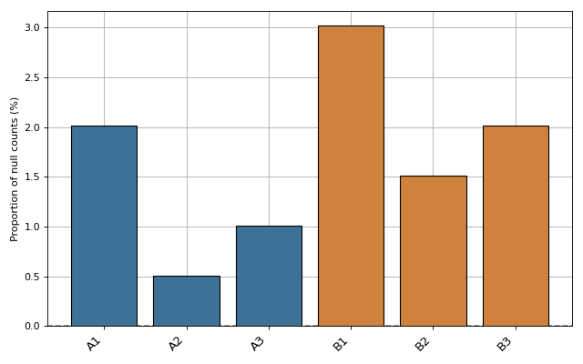

plot_upset(force=False, max_subsets=20)

Plot the upset plot (alternative to venn diagram).

with many comparisons, plots may be quite large. We can reduce the width by ignoring the small subsets. We fix the max number of subsets to 20 for now.

read_annot(gff)

Get a properly formatted dataframe from the gff.

Parameters:

gff -- a input GFF filename or an existing instance of GFF3

read_csv(filename)

report()

summary()

to_csv(filename)

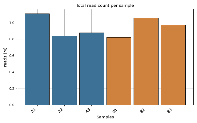
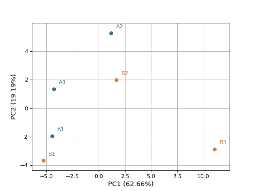
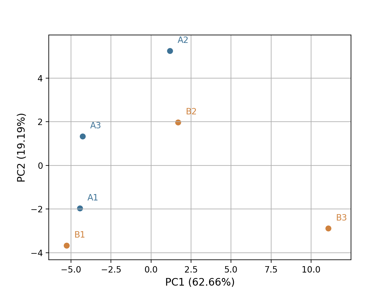
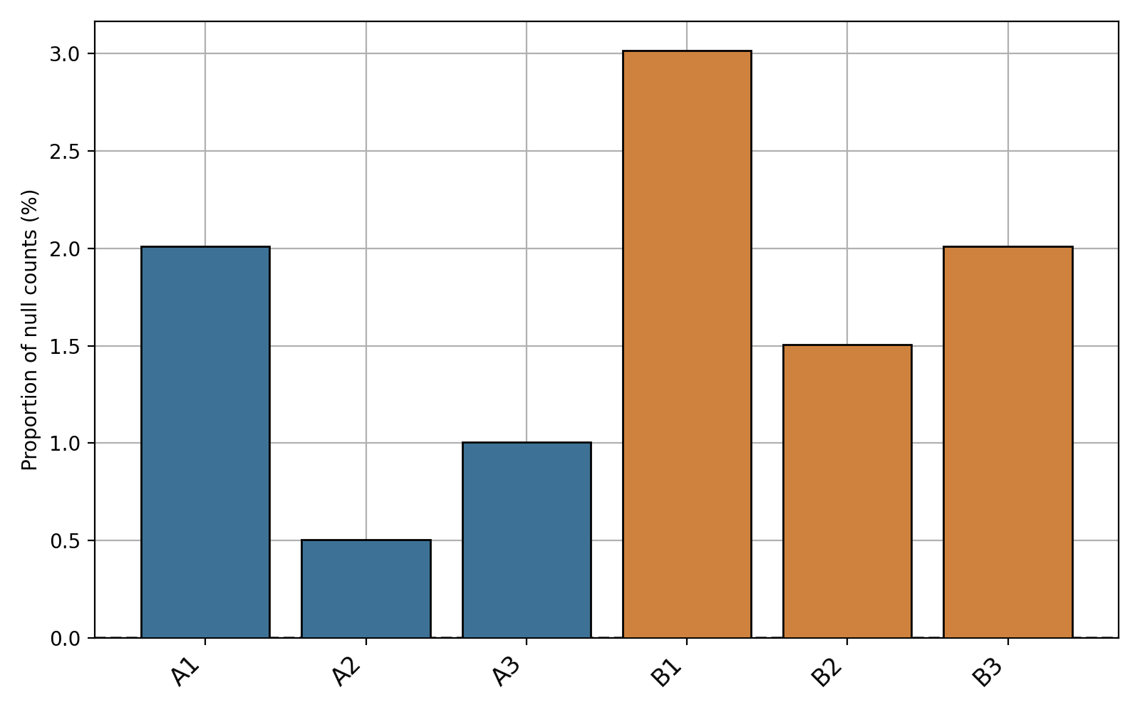
class RNADiffTable(path, alpha=0.05, log2_fc=0, sep=',', condition='condition', shrinkage=True)

A representation of the results of a single rnadiff comparison

Expect to find output of RNADiffAnalysis file named after condt1_vs_cond2_degs_DESeq2.csv

from sequana.rnadiff import RNADiffTable
RNADiffTable("A_vs_B_degs_DESeq2.csv")

property alpha

filter()

filter a DESeq2 result with FDR and logFC thresholds

property log2_fc

plot_padj_hist(bins=60, fontsize=16)

plot_pvalue_hist(bins=60, fontsize=16, rotation=0)

plot_volcano(padj=0.05, add_broken_axes=False, markersize=4, limit_broken_line=[20, 40], plotly=False, annotations=None, hover_name=None)

from sequana.rnadiff import RNADiffResults
from sequana import sequana_data

r = RNADiffResults(sequana_data("rnadiff/", "doc"))
r.comparisons["A_vs_B"].plot_volcano()

(Source code, png, hires.png, pdf)

set_gene_lists()

summary()

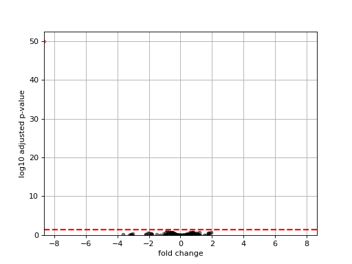
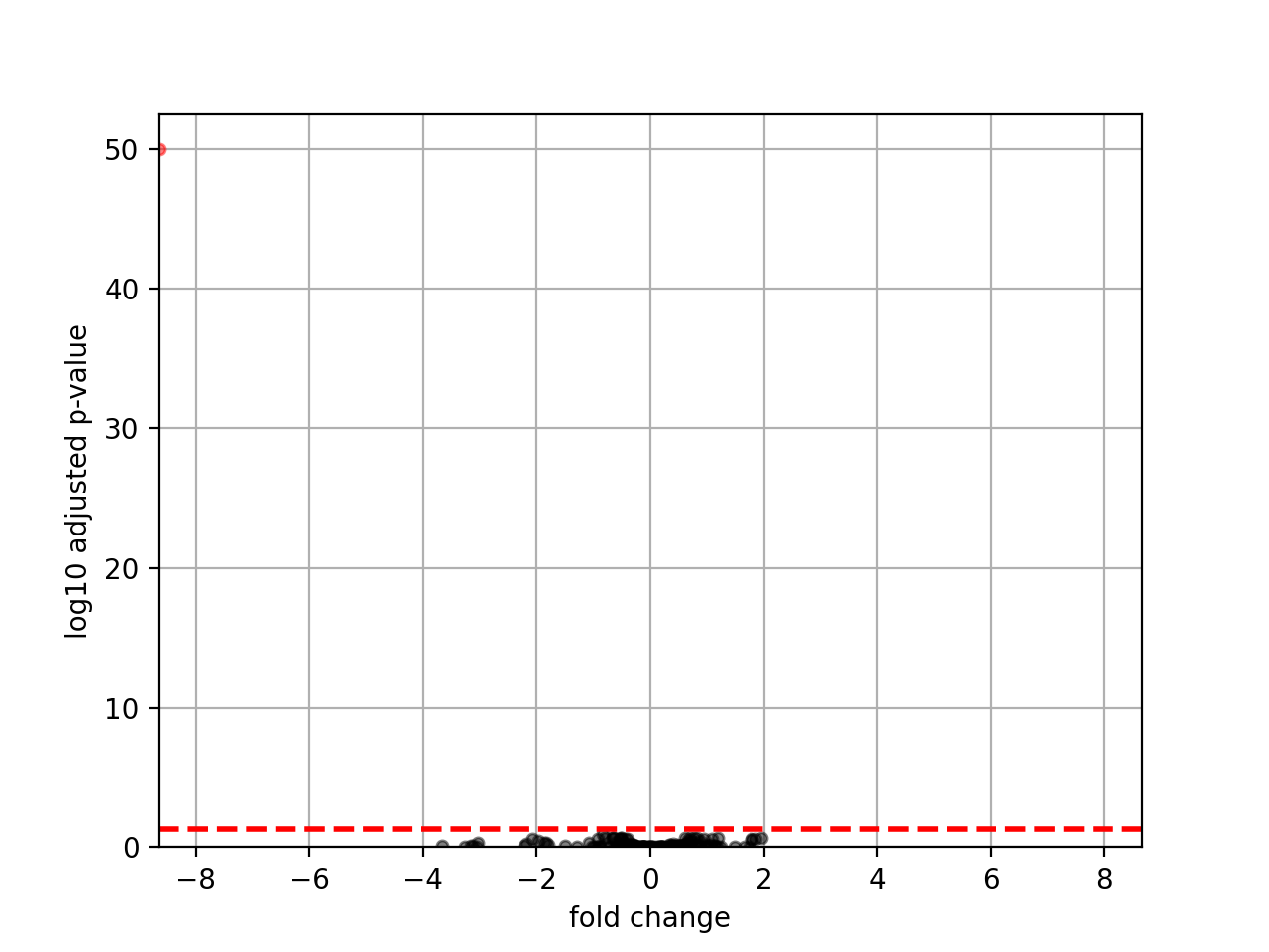
class RNADiffCompare(*args, design=None)

An object representation of results coming from a RNADiff analysis.

from sequana.compare import RNADiffCompare
c = RNADiffCompare("data.csv", "data2.csv")

# change the l2fc to update venn plots
c.plot_venn_up()
c.r1.log2_fc = 1
c.r2.log2_fc = 1
c.plot_venn_up()

plot_common_major_counts(mode, labels=None, switch_up_down_cond2=False, add_venn=True, xmax=None, title='', fontsize=12, sortby='log2FoldChange')

Parameters:

mode -- down, up or all

from sequana import sequana_data
from sequana.compare import RNADiffCompare

c = RNADiffCompare(
    sequana_data("rnadiff_salmon.csv", "doc/rnadiff_compare"),
    sequana_data("rnadiff_bowtie.csv", "doc/rnadiff_compare")
)
c.plot_common_major_counts("down")

(Source code, png, hires.png, pdf)

plot_corrplot_counts_normed(samples=None, log2=True, lower='pie', upper='text')

plot_corrplot_counts_raw(samples=None, log2=True, lower='pie', upper='text')

plot_foldchange()

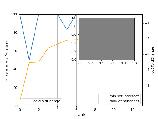
plot_geneset(indices, showlines=True, showdots=True, colors={'bodies': 'blue', 'cbars': 'k', 'cmaxes': 'k', 'cmins': 'k', 'dot': 'blue'})

indices is a list that represents a gene sets

cmins, cmaxes, cbars are the colors of the bars inside the body of the violin plots

(Source code, png, hires.png, pdf)

plot_jaccard_distance(mode, padjs=[0.0001, 0.001, 0.01, 0.05, 0.1], Nfc=50, smooth=False, window=5)

plot_venn_all(labels=None, ax=None, title='all expressed genes', mode='all')

plot_venn_down(labels=None, ax=None, title='Down expressed genes', mode='all', l2fc=0)

plot_venn_up(labels=None, ax=None, title='Up expressed genes', mode='all', l2fc=0)

Venn diagram of cond1 from RNADiff result1 vs cond2 in RNADiff result 2

from sequana import sequana_data
from sequana.compare import RNADiffCompare

c = RNADiffCompare(
    sequana_data("rnadiff_salmon.csv", "doc/rnadiff_compare"),
    sequana_data("rnadiff_bowtie.csv", "doc/rnadiff_compare")
)
c.plot_venn_up()

(Source code, png, hires.png, pdf)

plot_volcano(labels=None)

Volcano plot of log2 fold change versus log10 of adjusted p-value

from sequana import sequana_data
from sequana.compare import RNADiffCompare

c = RNADiffCompare(
    sequana_data("rnadiff_salmon.csv", "doc/rnadiff_compare"),
    sequana_data("rnadiff_bowtie.csv", "doc/rnadiff_compare")
)
c.plot_volcano()

(Source code, png, hires.png, pdf)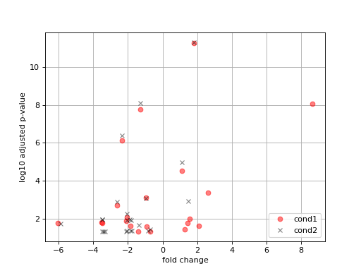

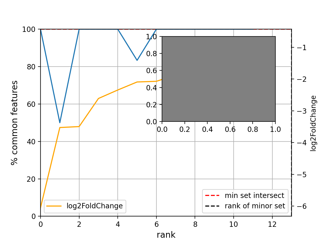
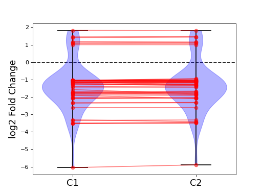
plot_volcano_differences(mode='all')

11.19. Running median

Data analysis tool

RunningMedian(data, width[, container])

Running median (fast)

class RunningMedian(data, width, container=<class 'list'>)

Running median (fast)

This is an efficient implementation of running median, faster than SciPy implementation v0.17 and a skip list method.

The main idea comes from a recipe posted in this website: http://code.activestate.com/recipes/576930/#c3 that uses a simple list as proposed in https://gist.github.com/f0k/2f8402e4dfb6974bfcf1 and was adapted to our needs included object oriented implementation.

Note

a circular running median is implemented in sequana.bedtools.SequanaCoverage

from sequana.running_median import RunningMedian
rm = RunningMedian(data, 101)
results = rm.run()

Warning

the first W/2 and last W/2 positions should be ignored since they do not use W values. In this implementation, the last W/2 values are currently set to zero.

This shows how the results agree with scipy

from pylab import *
import scipy.signal
from sequana.running_median import RunningMedian

clf()
x = randn(100)
plot(x, 'k')
plot(RunningMedian(x,9).run(), 'r', lw=4)
plot(scipy.signal.medfilt(x, 9), 'go')
grid()

(Source code, png, hires.png, pdf)

from sequana.running_median import RunningMedian
from pylab import *

N = 1000
X = linspace(0, N-1, N)

# Create some interesting data with SNP and longer over
# represented section.
data = 20 + randn(N) + sin(X*2*pi/1000.*5)
data[300:350] += 10
data[500:505] += 100
data[700] = 1000

plot(X, data, "k", label="data")
rm = RunningMedian(data, 101)
plot(X, rm.run(), 'r', label="median W=201")

from sequana.stats import moving_average as ma
plot(X[100:-100], ma(data, 201), 'g', label="mean W=201")
grid()
legend()
ylim([10, 50])

(Source code, png, hires.png, pdf)

Note that for visualisation, we set the ylimits to 50 but the data at position 500 goes up to 120 and there is an large outlier (1000) at position 700 .

We see that the median is less sensible to the outliers, as expected. The median is highly interesting for large outliers on short duration (e.g. here the peak at position 500) but is also less biases by larger regions.

Note

The beginning and end of the running median are irrelevant. There are actually equal to the data in our implementation.

Note

using blist instead of list is not always faster. It depends on the width of the window being used. list and blist are equivaltn for W below 20,000 (list is slightly faster). However, for large W, blist has an O(log(n)) complexity while list has a O(n) complexity

constructor

Parameters:

• data -- your data vector

• width -- running window length

• container -- a container (defaults to list). Could be a B-tree blist from the blist package but is 30% slower than a pure list for W < 20,000

scipy in O(n) list in sqrt(n) blist in O(log(n))

run()

running_median(data, width, container=<class 'list'>)

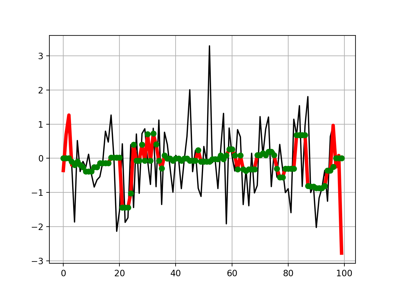
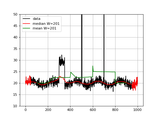
11.20. Snpeff module

Tools to launch snpEff.

class SnpEff(annotation, log=None, snpeff_datadir='data', fastafile=None, build_options='')

SnpEff is a tool dedicated to annotate detected variants in a VCF file. This wrapper eases the annotation with a genbank file. It create automatically the custom database. Then, run snpEff with a subprocess. Caution, the locus name (or chromosome name) in genbank file and the sequence name in VCF file must be the same. Otherwise, snpEff is not able to bind informations.

Example:

snpeff = SnpEff('file.gbk')
snpeff.launch_snpeff('variants.vcf', 'variant.ann.vcf')

If your input is in GFF format, you must also provide the fasta reference file.

Will save relevant snpeff data into ./data directory (or snpeff_datadir).

Constructor

Parameters:

• annotation -- annotation reference.

• file_format -- format of your file. ('only genbank actually')

• log -- log file

• snpeff_datadir -- default to data.

• fastafile -- if a GFF is used, you must provide the FASTA input file as well

add_locus_in_fasta(fasta, output_file)

Add locus of annotation file in description line of fasta file. If fasta file and genbank file do not have the same names.

Parameters:

• fasta (str) -- input fasta file where you want to add locus.

• output_file (str) -- output file.

FIXME: fasta is already known if provided in the init

launch_snpeff(vcf_filename, output, html_output=None, options='')

Launch snpEff with the custom genbank file.

Parameters:

• vcf_filename (str) -- input VCF filename.

• output (str) -- output VCF filename.

• html_output (str) -- filename of the HTML creates by snpEff.

• options (str) -- any options recognised by snpEff.

download_fasta_and_genbank(identifier, tag, genbank=True, fasta=True, outdir='.')

Parameters:

• identifier -- valid identifier to retrieve from NCBI (genbank) and ENA (fasta)

• tag -- name of the filename for the genbank and fasta files.

11.21. General tools

misc utilities

findpos(seq, chr)

Find position(s) of a substring into a longer string.

Note that this function is a generator:

>>> list(findpos("AACCGGAAGGTT", "GG"))
[4,8]

normpdf(x, mu, sigma)

Return the normal pdf evaluated at x; args provides mu, sigma"

Note

same as scipy.stats.norm but implemented to avoid scipy dependency

textwrap(text, width=80, indent=0)

Wrap a string with 80 characters

Parameters:

• text -- input text

• width -- (defaults to 80 characters)

• indent -- possible indentation (0 by default)

wget(link, output)

Retrieve a file from internet.

Parameters:

• link (str) -- a valid URL

• output (str) -- the output filename

Warning

no sanity check of any kind for now

General tools

class GZLineCounter(filename)

Fast GZipped line counter

Uses zcat if possible, otherwise gzip library (twice as slow).

>>> from sequana import sequana_data
>>> from sequana.tools import GZLineCounter
>>> gz = GZLineCounter(sequana_data("test.fastq.gz"))
>>> len(gz)
1000

class StatsBAM2Mapped(bamfile=None, wkdir=None, verbose=True)

to_html()

to_json(filename)

bam_to_mapped_unmapped_fastq(filename, output_directory=None, progress=True)

Create mapped and unmapped fastq files from a BAM file

Context:

given a reference, one or two FastQ files are mapped onto the reference to generate a BAM file. This BAM file is a compressed version of a SAM file, which interpretation should be eased within this function.

Parameters:

• filename -- input BAM file

• output_directory -- where to save the mapped and unmapped files

Returns:

dictionary with number of reads for each file (mapped/unmapped for R1/R2) as well as the mode (paired or not), the number of unpaired reads, and the number of duplicated reads. The unpaired reads should be zero (sanity check)

Given a BAM file, create FASTQ with R1/R2 reads mapped and unmapped. In the paired-end case, 4 files are created.

Note that this function is efficient in that it does not create intermediate files limiting IO in the process. As compared to standard tools such as bedtools bamtofastq, it is 1.5 to 2X slower but it does create the mapped AND unmapped reads.

Details:

Secondary alignment (flag 256) are dropped so as to remove any ambiguous alignments. The output dictionary stores "secondary" key to keep track of the total number of secondary reads that are dropped. If the flag is 256 and the read is unpaired, the key unpaired is also incremented.

If the flag is not equal to 256, we first reverse complement reads that are tagged as reverse in the BAM file. Then, reads that are not paired or not "proper pair" (neither flag 4 nor flag 8) are ignored.

If R1 is mapped or R2 is mapped then the reads are considered mapped. If both R1 and R2 are unmapped, then reads are unmapped.

Note

about chimeric alignment: one is the representative and the other is the supplementary. This flag is not used in this function. Note also that chimeric alignment have same QNAME and flag 4 and 8

Note

the contamination reported is based on R1 only.

Todo

comments are missing since there are not stored in the BAM file.

Note

the mapped reads may not be synchronized because we include also the chimeric alignment (cf samtools documentation). However, total reads = unmappeds reads + R1 mapped + R2 mapped - supplementary reads (those with flag 2048).

11.22. Peaks

class MACS3Reader(filename)

This class reads output of macs3 tool

from sequana import MACS3Reader
mr = MACS3Reader(data)
mr.df
mr.plot_volcano()

If input file ends in .xls, we assume this is a NAME_peaks.xls file. It is therefore a tabulated file where columns are:

• chromosome name

• start position of peak

• end position of peak

• length of peak region

• absolute peak summit position

• pileup height at peak summit

• -log10(pvalue) for the peak summit (e.g. pvalue =1e-10, then this value should be 10)

• fold enrichment for this peak summit against random Poisson distribution with local lambda,

• -log10(qvalue) at peak summit

Note that coordinates in XLS is 1-based which is different from BED format that follows. When --broad is enabled for broad peak calling, the pileup, p-value, q-value, and fold change in the XLS file will be the mean value across the entire peak region, since peak summit won't be called in broad peak calling mode.

NAME_peaks.narrowPeak is BED6+4 format file which contains the peak locations together with peak summit, p-value, and q-value.

The fifth column is the score calculate as int(-10*log10_pvalue) or int(-10*log10_pvalue) where log10-pvalue/log10-qvalue is the 8th or 9th column depending on whether -p (pvalue) or -q (qvalue) is used as score cutoff. The 7th columns stores the fold-change at peak summit. The 8th is -log10pvalue at peak summit and the 9th is -log10qvalue at peak summit. The 10th is the relative summit position to peak start equivalent to absolute peak summit position in the xls file.

NAME_peaks.broadPeak is in BED6+3 format which is similar to narrowPeak file, except for missing the 10th column for annotating peak summits. This file and the gappedPeak file will only be available when --broad is enabled. Since in the broad peak calling mode, the peak summit won't be called, the values in the 5th, and 7-9th columns are the mean value across all positions in the peak region. Refer to narrowPeak if you want to fix the value issue in the 5th column

plot_volcano(plotly=False, marker_color='b', title='')

Plots -log10 p-value versus fold change of all peaks

class PeakConsensus(f1, f2)

merge(overlap=0.2)

plot_venn(title='', labels=[])

to_bed(filename)

to_saf(filename)

For now, all strand are categorised as strand + . strand not used in the pipeline for now.

11.23. Format IO

class BED(filename)

a structure to read and manipulate BED files (12-column file)

columns are defined as chromosome name, start and end, gene_name, score, strand, CDS start and end, blcok count, block sizes, block starts:

get_CDS_exons()

Extract CDS from input BED file.

get_exons()

Extract exon regions from input BED file.

Uses the first (chromosome name), second (chromosome start), 11th and 12th columns (exon start and size) of a 12-columns BED file.

from sequana import sequana_data
from sequana import BED
b = BED(sequana_data("hg38_chr18.bed"))
b.get_exons()

get_transcript_ranges()

Extract transcript from input BED file.

class GFF3(filename, skip_types=['biological_region'])

Read a GFF file, version 3

See also

https://github.com/The-Sequence-Ontology/Specifications/blob/master/gff3.md

g = GFF3(filename)
# first call is slow
g.df
# print info about the different feature types
g.features
# prints info about duplicated attributes:
g.get_duplicated_attributes_per_genetic_type(self)

On eukaryotes, the reading and processing of the GFF may take a while. On prokaryotes, it should be pretty fast (a few seconds). To speed up the eukaryotes case, we skip the processing biological_regions (50% of the data in mouse).

property attributes

Return list of possible attributes

If feature is provided, must be valid and used as a filter to keep only entries for that feature.

~10 seconds on mouse genome GFF file.

sep must be "; " with extra space to cope with special cases where an attribute has several entries separated by ; e.g.:

BP="GO:0006412"; MF="GO:0005524;GO:0004004;"

clean_gff_line_special_characters(text)

Simple leaner of gff lines that may contain special characters

property df

property features

Extract unique GFF feature types

This is equivalent to awk '{print $3}' | sort | uniq to extract unique GFF types. No sanity check, this is suppose to be fast.

Less than a few seconds for mammals.

get_attributes(feature=None, sep='; ')

Return list of possible attributes

If feature is provided, must be valid and used as a filter to keep only entries for that feature.

~10 seconds on mouse genome GFF file.

sep must be "; " with extra space to cope with special cases where an attribute has several entries separated by ; e.g.:

BP="GO:0006412"; MF="GO:0005524;GO:0004004;"

get_duplicated_attributes_per_genetic_type()

get_features_dict()

Format feature dict for sequana_coverage.

get_simplify_dataframe()

Method to simplify the gff and keep only the most informative features.

read()

Read annotations one by one creating a generator

read_and_save_selected_features(outfile, features=['gene'])

save_annotation_to_csv(filename='annotations.csv')

save_gff_filtered("test.gff", features=['misc_RNA', 'rRNA'], replace_seqid='locus_tag')

to_bed(output_filename, attribute_name)

Experimental export to BED format to be used with rseqc scripts

Parameters:

attribute_name (str) -- the attribute_name name to be found in the GFF attributes

to_fasta(ref_fasta, fasta_out)

From a genomic FASTA file ref_fasta, extract regions stored in the gff. Export the corresponding regions to a FASTA file fasta_out.

Parameters:

• ref_fasta -- path to genomic FASTA file to extract rRNA regions from.

• fasta_out -- path to FASTA file where rRNA regions will be exported to.

to_gtf(output_filename='test.gtf', mapper={'ID': '{}_id'})

transcript_to_gene_mapping(feature='all', attribute='transcript_id')

Parameters:

• feature -- not used yet

• attribute -- the attribute to be usde. should be transcript_id for salmon compatability but could use soething different.

11.24. VCF module

11.25. Module Reports

Generic module is the parent module of all other module

class SequanaBaseModule(template_fn='standard.html', required_dir=None)

Generic Module to write HTML reports.

# to add a TOC, add this code:

<div id="tocDiv">
<ul id="tocList"> </ul>
</div>

add_code_section(content, language)

Add code in your html.

add_float_right(content)

Align a content to right.

add_fotorama(files, width=600, height=800, loop=True, thumbnails=True, file_thumbnails=None, captions=None)

copy_file(filename, target_dir)

Copy a file to a target directory in report dir. Return the relative path of your file.

Parameters:

• filename (str) -- file to copy.

• target_dir (str) -- directory where to copy.

Return relative path of the new file location.

create_combobox(path_list, html_id, newtab=True)

Create a dropdown menu with QueryJS.

Parameters:

path_list (list) -- list of links.

return html div and js script as string.

create_embedded_png(plot_function, input_arg, style=None, **kwargs)

Take as a plot function as input and create a html embedded png image. You must set the arguments name for the output to connect buffer.

create_hide_section(html_id, name, content, hide=False)

Create an hideable section.

Parameters:

• html_id (str) -- add short id to connect all elements.

• name (str) -- name of the hyperlink to hide or display the content.

• content (str) -- hideable HTML content.

• hide (bool) -- set if the first state is hiding or not.

Return tuple that contains HTML hyperlink and hideable section.

create_html(output_filename)

Create HTML file with Jinja2.

Parameters:

output_filename (str) -- HTML output filename

create_link(name, target, newtab=True, download=False)

Create an HTML hyperlink with name and target.

Parameters:

• target (str) -- the target url.

• newtab (bool) -- open html page in a new tab.

• download (bool) -- download the target.

Return as string the HTML hyperlink to the target.

include_svg_image(filename, alt='undefined')

Include SVG image in the html.

png_to_embedded_png(png, style=None, alt='', title='')

Include a PNG file as embedded file.

Report dedicated to BAM file

BAMQCModule(bam_input[, output_filename])

Report dedicated to BAM file

class BAMQCModule(bam_input, output_filename=None)

Report dedicated to BAM file

from sequana import sequana_data
from sequana.modules_report.bamqc import BAMQCModule
filename = sequana_data("test.bam")

r = BAMQCModule(filename)
r.create_html("test.html")

# report/bam.html is now available

Todo

right now, the computation is performed in the class. Ideally, we would like the computation to happen elsewhere, where a json is stored. The json would be the input to this class.

add_flag_section()

add_images_section()

create_report_content()

Module to write coverage report

class ChromosomeCoverageModule(chromosome, datatable, region_window=200000, options=None, command='', skip_html=False)

Write HTML report of coverage analysis for each chromosome. It is created by CoverageModule.

Parameters:

• chromosome --

• datatable --

• directory --

• region_window (int) -- length of the sub coverage plot

• options -- should contain "W", "k", "circular"

add_command()

basic_stats()

Basics statistics section.

coverage_barplot()

Coverage barplots section.

coverage_plot()

Coverage section.

create_report_content(directory, options=None)

Generate the sections list to fill the HTML report.

gc_vs_coverage()

3 dimensional plot of GC content versus coverage.

normalized_coverage()

Barplot of normalized coverage section.

regions_of_interest(rois, links)

Region of interest section.

subcoverage(rois, directory)

Create subcoverage reports to have access to a zoomable line plot.

Params rois:

Parameters:

directory -- directory name for the chromsome

This method create sub reports for each region of 200,000 bases (can be changed). Usually, it starts at position 0 so reports will be stored in e.g. for a genome of 2,300,000 bases:

chromosome_name/chromosome_name_0_200000.html
chromosome_name/chromosome_name_200000_400000.html
...
...
chromosome_name/chromosome_name_2000000_2200000.html
chromosome_name/chromosome_name_2200000_2300000.html

Note that if the BED file positions does not start at zero, then names will take care of that.

zscore_distribution()

Barplot of zscore distribution section.

class CoverageModule(data, region_window=200000)

Write HTML report of coverage analysis. This class takes either a SequanaCoverage instances or a csv file where analysis are stored.

constructor

Parameters:

• data -- it can be a csv filename created by sequana_coverage or a bedtools.SequanaCoverage object.

• region_window --

create_chromosome_reports()

Create HTML report for each chromosome present in data.

create_chromosome_table(html_list)

Create table with links to chromosome reports

init_roi_datatable()

Initiate DataTableFunction to create table to link each row with sub HTML report. All table will have the same appearance. We can therefore initialise the roi once for all.

Parameters:

rois -- can be a ROIs from ChromosomeCov instance or a simple dataframe

11.26. Wrapper to other tools

class ITOL(tree, APIkey=None, projectName=None)

Tree with branch lengths:

(A:0.1,(B:0.1,C:0.1)));

Tree with bootstrap and branch lengths:

(A:0.1,(B:0.1,C:0.1)90:0.1)98:0.3);

from pylab import imshow, imread
from easydev import TempFile
from sequana import ITOL, sequana_data

# You mut have an APIkey and project name defined on itol web site.
itol = ITOL(sequana_data("test_itol_basic.tree.txt"), APIkey, projectName)
itol.upload()
# You can change the parameters in itol.params
itol.params["display_mode"] = 1  # use linear layout instead of circular

# finally export your image locally:
with TempFile(suffix=".png") as fout:
    itol.export(fout.name)
    imshow(imread(fout.name))

For details, please see https://itol.embl.de/help.cgi#annot Here are some parameters:

• display_mode: 1,2 or 3 (1=rectangular, 2=circular, 3=unrooted)

constructor

add_file(filename)

export(filename='test.png', extra_params={}, tree_id=None, circular=True)

Export or retrieve an existing tree to get back the resulting image

Parameters:

• filename (str) -- the filename where to store the image

• extra_params -- parameters use to tune the trre are stored in params but you may provide extra parameters here ot alter some. If you this paramterm, the main attribute params is unchanged.

• tree_id -- if you have a known tree identifier, you can retrieve it using the tree_id parameter. Otherwise, if you have just uploaded a tree with upload(), the identifier is automatically populated and that is the tree you will export.

upload()

class CNVnator(filename)

Reader of the CNVnator output file.

hist_event_size(bins=20)

plot(chr_name, x1=None, x2=None, Y=20)

class CanuScanner(path='.')

getfile(filename)

hist_read_length(bins=100, fontsize=16)

hist_read_length2(fontsize=16)

hist_trimming_read_length(bins=100, fontsize=16)

plot_correction_check1(alpha=0.5)

plot_kmer(bins=100)

scan_correction()

scan_trimming()

set_overlap_filtering()

set_read_correction()

class StatsFile(filename='Stats.json')

Reads a bcl2fastq Stats.json file and produces useful plots for QCs

barplot(filename='lane{}_status.png', lanes=None)

barplot_per_sample(alpha=0.5, width=0.8, filename=None)

barplot_summary(filename=None, color=['green', 'red'], alpha=0.8)

get_data_reads()

plot_unknown_barcodes(N=20)

to_summary_reads(filename)

class TRF(filename, verbose=False, frmt=None)

Tandem Repeat Finder utilities

The input data is the output of trf tool when using the -d option. This is not a CSV file. It contains comments in the middle of the file to indicate the name of the contig.

The output filename has the following filename convention:

test.fa.2.5.7.80.10.50.2000.dat

where the numbers indicate the 7 input parameters:

• Match = matching weight

• Mismatch = mismatching penalty

• Delta = indel penalty

• PM = match probability (whole number)

• PI = indel probability (whole number)

• Minscore = minimum alignment score to report

• MaxPeriod = maximum period size to report

You may use -h to suppress html output.

Then, you can use this class to easly identify the pattern you want:

t = TRF("input.dat")
query = "length>100 and period_size==3 and entropy>0 and C>20 and A>20 and G>20"
t.df.query(query)

hist_cnvs(bins=50, CNVmin=10, motif=['CAG', 'AGC', 'GCA'], color='r', log=True)

histogram of the motif found in the list provided by users. As an example, this is triplet CAG. Note that we also add the shifted version AGC and GCA.

hist_entropy(bins=50)

Histogram of the entropy of all found repeats

hist_length_repetition(bins=50, CNVmin=3, motif=['CAG', 'AGC', 'GCA'], color='r', log=True)

histogram of the motif found in the list provided by users. As an example, this is triplet CAG. Note that we also add the shifted version AGC and GCA.

hist_period_size(bins=50)

Length of the repetitions

hist_repet_by_sequence()

scandata(verbose=True, max_seq_length=20)

scan output of trf and returns a dataframe

The format of the output file looks like:

Tandem Repeats Finder Program

some info

Sequence: chr1

Parameters: 2 5 7 80 10 50 2000

10001 10468 6 77.2 6 95 3 801 33 51 0 15 1.43 TAACCC TAACCCTA...
1 10 6 77.2 6 95 3 801 33 51 0 15 1.43 TAACCC TAACCCTA...

Sequence: chr2

Parameters: 2 5 7 80 10 50 2000

10001 10468 6 77.2 6 95 3 801 33 51 0 15 1.43 TAACCC TAACCCTA...

The dataframe stores a row for each sequence and each pattern found. For instance, from the example above you will obtain 3 rows, two for the first sequence, and one for the second sequence.

11.27. Misc

Retrieve data from sequana library

sequana_data(filename=None, where=None)

Return full path of a sequana resource data file.

Parameters:

• filename (str) -- a valid filename to be found

• where (str) -- one of the registered data directory (see below)

Returns:

the path of file. See also here below in the case where filename is set to "*".

from sequana import sequana_data
filename = sequana_data("test.fastq")

Type the function name with "*" parameter to get a list of available files. Withe where argument set, the function returns a list of files. Without the where argument, a dictionary is returned where keys correspond to the registered directories:

filenames = sequana_data("*", where="images")

Registered directories are:

• data

• testing

• images

Note

this does not handle wildcards. The * means retrieve all files.

Some useful data sets to be used in the analysis

The command sequana.sequana_data() may be used to retrieved data from this package. For example, a small but standard reference (phix) is used in some NGS experiments. The file is small enough that it is provided within sequana and its filename (full path) can be retrieved as follows:

from sequana import sequana_data
fullpath = sequana_data("phiX174.fa", "data")

Other files stored in this directory will be documented here.

adapters = {'adapters_netflex_pcr_free_1_fwd': 'adapters_netflex_pcr_free_1_fwd.fa', 'adapters_netflex_pcr_free_1_rev': 'adapters_netflex_pcr_free_1_rev.fa'}

List of adapters used in various sequencing platforms

Sniffer

sniffer(filename)

Utilities to create a Jquery DataTable for your HTML file.

DataTableFunction(df, html_id[, index])	Class that contains Jquery DataTables function and options.
DataTable(df, html_id[, datatable, index])	Class that contains html table which used a javascript function.

class DataTable(df, html_id, datatable=None, index=False)

Class that contains html table which used a javascript function.

You must add in your HTML file the JS function (DataTable.create_javascript_function()) and the HTML code (DataTable.create_datatable()).

Example:

df = pandas.read_csv('data.csv')
datatable = DataTable(df, 'data')
datatable.datatable.datatable_options = {'pageLength': 15,
                                         'dom': 'Bfrtip',
                                         'buttons': ['copy', 'csv']}
js = datatable.create_javascript_function()
html = datatable.create_datatable()

# Second CSV file with same format
df2 = pandas.read_csv('data2.csv')
datatable2 = DataTable(df2, 'data2', datatable.datatable)
html2 = datatable.create_datatable()

The reason to include the JS manually is that you may include many HTML table but need to include the JS only once.

contructor

Parameters:

• df -- data frame.

• html_id (str) -- the unique ID used in the HTML file.

• datatable (DataTableFunction) -- javascript function to create the Jquery Datatables. If None, a DataTableFunction is generated from the df.

• index (bool) -- indicates whether the index dataframe should be shown

create_datatable(style='width:100%', **kwargs)

Return string well formated to include in a HTML page.

Parameters:

• style (str) -- CSS option of your table.

• kwargs (dict) -- parameters of pandas.DataFrame.to_csv().

create_javascript_function()

Generate the javascript function to create the DataTable in a HTML page.

property df

property html_id

class DataTableFunction(df, html_id, index=False)

Class that contains Jquery DataTables function and options.

Example:

import pandas as pd
from sequana.utils.datatables_js import DataTableFunction

df = pandas.read_csv('data.csv')
datatable_js = DataTableFunction(df, 'data')
datatable_js.datatable_options = {'pageLength': 15,
                                  'dom': 'Bfrtip',
                                  'buttons': ['copy', 'csv']}
js = datatable_js.create_javascript_function()
html_datatables = [DataTable(df, "data_{0}".format(i), datatable_js)
                   for i, df in enumerate(df_list)]

Here, the datatable_options dictionary is used to fine tune the appearance of the table.

Note

DataTables add a number of elements around the table to control the table or show additional information about it. There are controlled by the order in the document (DOM) defined as a string made of letters, each of them having a precise meaning. The order of the letter is important. For instance if B is first, the buttons are put before the table. If B is at the end, it is shown below the table. Here are some of the valid letters and their meaning:

• B: add the Buttons (copy/csv)

• i: add showing 1 to N of M entries

• f: add a search bar (f filtering)

• r: processing display element

• t: the table itself

• p: pagination control

Each option can be specified multiple times (with the exception of the table itself).

Note

other useful options are:

• pageLength: 15

• scrollX: "true"

• paging: 15

• buttons: ['copy', 'csv']

Note that buttons can also be excel, pdf, print, ...

All options of datatable:

https://datatables.net/reference/option/

contructor

Parameters:

• df -- data frame.

• html_id (str) -- the ID used in the HTML file.

create_javascript_function()

Return javascript to create the DataTable.

property datatable_columns

Get datatable_columns dictionary. It is automatically set from the dataframe you want to plot.

property datatable_options

Get, set or delete the DataTable options. Setter takes a dict as parameter with the desired options and updates the current dictionary.

Example:

datatable = DataTableFunction("tab")
datatable.datatable_options = {'dom': 'Bfrtip',
                               'buttons': ['copy', 'csv']}

source: https://datatables.net/reference/option/

property html_id

Get the html_id, which cannot be set by the user after the instanciation of the class.

set_links_to_column(link_col, target_col, new_page=True)

Hide a column with urls and connect it with a column.

Parameters:

• link_col (str) -- column with your URLs.

• target_col (str) -- column to connect.

set_tooltips_to_column(tooltips_col, target_col)

Hide a column with tooltips and connect it with a column.

Parameters:

• tooltips_col (str) -- column with your tooltips.

• target_col (str) -- column to connect.